steve_bank
Diabetic retinopathy and poor eyesight. Typos ...
https://en.wikipedia.org/wiki/Central_limit_theorem
The CLT is a foundation for practical statistical analysis and sampling methods. It leads to the sampling distribution of the mean.
https://stats.libretexts.org/Booksh..._The_Sampling_Distribution_of_the_Sample_Mean
And confidence intervals
https://en.wikipedia.org/wiki/Confidence_int
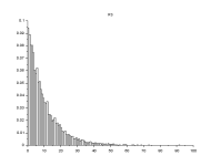
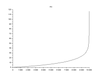
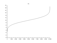
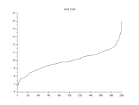
The code takes the average of a sample size through a random vector. Sort asscebding gives a cumulative distribution.
clear
samp_size = 50
N = 10000
Nsamp = N/samp_size
r = grand(N,1,"nor",10,3)
//r = grand(N,1,"exp",10)
rs = gsort(r,'g','i')
index = 0
for i = 1:Nsamp
acc = 0
for j = 1:samp_size
acc = acc + r(index + j )
end
s(i) =acc
index = index + samp_size-1
avg(i) =acc/samp_size
end
avgs = gsort(avg,'g','i')
In probability theory, the central limit theorem (CLT) establishes that, in many situations, when independent random variables are summed up, their properly normalized sum tends toward a normal distribution (informally a bell curve) even if the original variables themselves are not normally distributed. The theorem is a key concept in probability theory because it implies that probabilistic and statistical methods that work for normal distributions can be applicable to many problems involving other types of distributions. This theorem has seen many changes during the formal development of probability theory. Previous versions of the theorem date back to 1811, but in its modern general form, this fundamental result in probability theory was precisely stated as late as 1920,[1] thereby serving as a bridge between classical and modern probability theory.
For example, suppose that a sample is obtained containing many observations, each observation being randomly generated in a way that does not depend on the values of the other observations, and that the arithmetic mean of the observed values is computed. If this procedure is performed many times, the central limit theorem says that the probability distribution of the average will closely approximate a normal distribution. A simple example of this is that if one flips a coin many times, the probability of getting a given number of heads will approach a normal distribution, with the mean equal to half the total number of flips. At the limit of an infinite number of flips, it will equal a normal distribution.
The central limit theorem has several variants. In its common form, the random variables must be identically distributed. In variants, convergence of the mean to the normal distribution also occurs for non-identical distributions or for non-independent observations, if they comply with certain conditions.
The earliest version of this theorem, that the normal distribution may be used as an approximation to the binomial distribution, is the de Moivre–Laplace theorem.
The CLT is a foundation for practical statistical analysis and sampling methods. It leads to the sampling distribution of the mean.
https://stats.libretexts.org/Booksh..._The_Sampling_Distribution_of_the_Sample_Mean
And confidence intervals
https://en.wikipedia.org/wiki/Confidence_int
Philosophical issues
The principle behind confidence intervals was formulated to provide an answer to the question raised in statistical inference of how to deal with the uncertainty inherent in results derived from data that are themselves only a randomly selected subset of a population. There are other answers, notably that provided by Bayesian inference in the form of credible intervals. Confidence intervals correspond to a chosen rule for determining the confidence bounds, where this rule is essentially determined before any data are obtained, or before an experiment is done. The rule is defined such that over all possible datasets that might be obtained, there is a high probability ("high" is specifically quantified) that the interval determined by the rule will include the true value of the quantity under consideration. The Bayesian approach appears to offer intervals that can, subject to acceptance of an interpretation of "probability" as Bayesian probability, be interpreted as meaning that the specific interval calculated from a given dataset has a particular probability of including the true value, conditional on the data and other information available. The confidence interval approach does not allow this since in this formulation and at this same stage, both the bounds of the interval and the true values are fixed values, and there is no randomness involved. On the other hand, the Bayesian approach is only as valid as the prior probability used in the computation, whereas the confidence interval does not depend on assumptions about the prior probability.
The code takes the average of a sample size through a random vector. Sort asscebding gives a cumulative distribution.
clear
samp_size = 50
N = 10000
Nsamp = N/samp_size
r = grand(N,1,"nor",10,3)
//r = grand(N,1,"exp",10)
rs = gsort(r,'g','i')
index = 0
for i = 1:Nsamp
acc = 0
for j = 1:samp_size
acc = acc + r(index + j )
end
s(i) =acc
index = index + samp_size-1
avg(i) =acc/samp_size
end
avgs = gsort(avg,'g','i')

