steve_bank
Diabetic retinopathy and poor eyesight. Typos ...
Working solutions to c;calculating math functions.
#Python sin Taylor series
import math as ma
import array as ar
import numpy as np
from numpy.linalg import inv
import matplotlib.pyplot as plt
import warnings

# table 1/n! n = 1,3,5.....
factab = [
       1.0,
        0.16666666666666666,
        0.008333333333333333,
        0.0001984126984126984,
        2.7557319223985893e-06,
        2.505210838544172e-08,
        1.6059043836821613e-10,
        7.647163731819816e-13,
        2.8114572543455206e-15,
        8.22063524662433e-18,
        1.9572941063391263e-20,
        3.8681701706306835e-23,
        6.446950284384474e-26,
        9.183689863795546e-29,
        1.1309962886447718e-31,
        1.2161250415535181e-34,
        1.151633562077195e-37,
        9.67759295863189e-41,
        7.265460179153071e-44,
        4.902469756513544e-47,
        2.9893108271424046e-50,
        1.6552108677421951e-53,
        8.359650847182804e-57,
        3.866628513960594e-60,
        1.643974708316579e-63,
        6.446959640457174e-67,
        2.3392451525606576e-70,
        7.876246304918039e-74,
        2.4674957095607893e-77,
        7.210682961895936e-81,
        1.9701319568021682e-84,
        5.043860616493007e-88,
        1.2124664943492803e-91,
        2.74189618803546e-95,
        5.843768516699617e-99,
        1.1758085546679308e-102,
        2.2370786808750587e-106,
        4.030772397973078e-110,
        6.887854405285506e-114,
        1.117795262136564e-117,
        1.724992688482352e-121,
        2.53451761457883e-125,
        3.549744558233656e-129,
        4.7443792545223946e-133,
        6.057685462873333e-137,
        7.396441346609687e-141,
        8.64474210683694e-145,
        9.680562269694223e-149,
        1.039579281539328e-152,
        1.0715102881254669e-156]

def sin_taylor(x):
    n = 50
    k = 1
    s = 0
    for i in range(n):
        # i even add term else subtract term
        if (i% 2) == 0:
             s += pow(x,k)*factab[i]
        else:
            s -= pow(x,k)*factab[i]
        k += 2
    return s


n = 20
xmax = ma.pi*2  # sin() 360 degrees
x = np.ndarray(shape=(n,1),dtype = np.float64)
y = np.ndarray(shape=(n),dtype = np.float64)  # interpolated sin
ys = np.ndarray(shape=(n),dtype = np.float64) # sin() library function
x = np.linspace(0,xmax,n)  # 2*pi radians

print("sin taylor")
for i in range(n):
    y[i] = sin_taylor(x[i])
    ys[i] = ma.sin(x[i])
    print("%2.8f  %+2.15f   %+2.15f" %(x[i],ys[i],y[i]))


[fig, ax] = plt.subplots()
ax.plot(x, y, linewidth=2.0,color='r')
ax.plot(x, ys, linewidth=2.0,color='k')
ax.grid(color='k', linestyle='-', linewidth=2)
plt.show()x radians library sin() Taylor series
0.00000000 +0.0000000000000000 +0.0000000000000000
0.33069396 +0.3246994692046835 +0.3246994692046835
0.66138793 +0.6142127126896678 +0.6142127126896678
0.99208189 +0.8371664782625285 +0.8371664782625283
1.32277585 +0.9694002659393304 +0.9694002659393303
1.65346982 +0.9965844930066698 +0.9965844930066700
1.98416378 +0.9157733266550575 +0.9157733266550577
2.31485774 +0.7357239106731317 +0.7357239106731318
2.64555171 +0.4759473930370737 +0.4759473930370737
2.97624567 +0.1645945902807340 +0.1645945902807341
3.30693964 -0.1645945902807338 -0.1645945902807332
3.63763360 -0.4759473930370735 -0.4759473930370736
3.96832756 -0.7357239106731313 -0.7357239106731308
4.29902153 -0.9157733266550573 -0.9157733266550566
4.62971549 -0.9965844930066698 -0.9965844930066703
4.96040945 -0.9694002659393305 -0.9694002659393290
5.29110342 -0.8371664782625288 -0.8371664782625288
5.62179738 -0.6142127126896680 -0.6142127126896658
5.95249134 -0.3246994692046837 -0.3246994692046831
6.28318531 -0.0000000000000002 +0.0000000000000099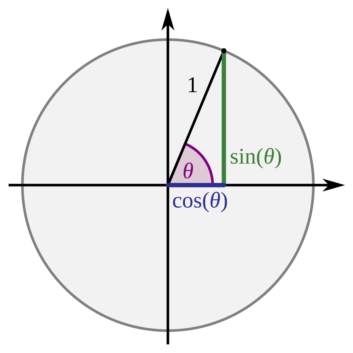
Code from the link. The code works only in the 1st quadrant 0-pi/2 or 90 degrees. The input x would gave to be processed to find the quadrant for x>pi/2 ro make it work 0-2*pi.CORDIC (for "coordinate rotation digital computer"), also known as Volder's algorithm, or: Digit-by-digit method Circular CORDIC (Jack E. Volder),[1][2] Linear CORDIC, Hyperbolic CORDIC (John Stephen Walther),[3][4] and Generalized Hyperbolic CORDIC (GH CORDIC) (Yuanyong Luo et al.),[5][6] is a simple and efficient algorithm to calculate trigonometric functions, hyperbolic functions, square roots, multiplications, divisions, and exponentials and logarithms with arbitrary base, typically converging with one digit (or bit) per iteration. CORDIC is therefore also an example of digit-by-digit algorithms. CORDIC and closely related methods known as pseudo-multiplication and pseudo-division or factor combining are commonly used when no hardware multiplier is available (e.g. in simple microcontrollers and FPGAs), as the only operations it requires are additions, subtractions, bitshift and lookup tables. As such, they all belong to the class of shift-and-add algorithms. In computer science, CORDIC is often used to implement floating-point arithmetic when the target platform lacks hardware multiply for cost or space reasons.
from math import atan2, sqrt, sin, cos, radians
import math as ma
import array as ar
import numpy as np
from numpy.linalg import inv
import matplotlib.pyplot as plt
import warnings


ITERS = 100
theta_table = [atan2(1, 2**i) for i in range(ITERS)]

def compute_K(n):
    """
    Compute K(n) for n = ITERS. This could also be
    stored as an explicit constant if ITERS above is fixed.
    """
    k = 1.0
    for i in range(n):
        k *= 1 / sqrt(1 + 2 ** (-2 * i))
    return k

def CORDIC(alpha, n):
    K_n = compute_K(n)
    theta = 0.0
    x = 1.0
    y = 0.0
    P2i = 1  # This will be 2**(-i) in the loop below
    for arc_tangent in theta_table:
        sigma = +1 if theta < alpha else -1
        theta += sigma * arc_tangent
        x, y = x - sigma * y * P2i, sigma * P2i * x + y
        P2i /= 2
    return x * K_n, y * K_n

n = 20
xmax = ma.pi/2  # sin() 360 degrees
x = np.ndarray(shape=(n,1),dtype = np.float64)
y = np.ndarray(shape=(n),dtype = np.float64)  # interpolated sin
ys = np.ndarray(shape=(n),dtype = np.float64) # sin() libray function
yc = np.ndarray(shape=(n),dtype = np.float64) # sin() libray function
x = np.linspace(0,xmax,n)  # 2*pi raduans


for i in range(n):
     yc[i], y[i] = CORDIC(x[i], ITERS)
     #y[i] = sinx
     ys[i] = ma.sin(x[i])
     print("%2.8f  %+2.16f   %+2.16f" %(x[i],ys[i],y[i]))


[fig, ax] = plt.subplots()
ax.plot(x, y, linewidth=2.0,color='r')
ax.plot(x, ys, linewidth=2.0,color='k')
ax.plot(x, yc, linewidth=2.0,color='k')
ax.grid(color='k', linestyle='-', linewidth=2)
plt.show()x, sin(), CORDIC
0.00000000 +0.0000000000000000 +0.0000000000000000
0.08267349 +0.0825793454723323 +0.0825793454723323
0.16534698 +0.1645945902807339 +0.1645945902807339
0.24802047 +0.2454854871407991 +0.2454854871407992
0.33069396 +0.3246994692046835 +0.3246994692046835
0.41336745 +0.4016954246529694 +0.4016954246529693
0.49604095 +0.4759473930370735 +0.4759473930370735
0.57871444 +0.5469481581224268 +0.5469481581224267
0.66138793 +0.6142127126896678 +0.6142127126896681
0.74406142 +0.6772815716257410 +0.6772815716257410
0.82673491 +0.7357239106731316 +0.7357239106731317
0.90940840 +0.7891405093963936 +0.7891405093963936
0.99208189 +0.8371664782625285 +0.8371664782625287
1.07475538 +0.8794737512064891 +0.8794737512064885
1.15742887 +0.9157733266550574 +0.9157733266550580
1.24010236 +0.9458172417006346 +0.9458172417006353
1.32277585 +0.9694002659393304 +0.9694002659393305
1.40544935 +0.9863613034027223 +0.9863613034027227
1.48812284 +0.9965844930066698 +0.9965844930066698
1.57079633 +1.0000000000000000 +0.9999999999999999
from math import atan2, sqrt, sin, cos, radians
import math as ma
import array as ar
import numpy as np
from numpy.linalg import inv
import matplotlib.pyplot as plt
import warnings

#--------------------------------------------------------------
def shaft_angle(volts, n):
    # sensor roration 0-360 degrees  0-12 volts
    alpha = 0.
    ang = 2*ma.pi*volts/12.  #angle in radiabs
    sgn = 1
    if(ang > 0. and ang <= ma.pi/2):   #1st quadrant
        sgn = 1.
        alpha = ang
    if(ang > ma.pi/2. and ang <= 2*ma.pi):  #2nd quadrant
        sgn = 1.
        alpha = ma.pi - ang ;
    if(ang > ma.pi and ang <= 1.5*ma.pi): #3rd quadrant
        sgn = -1.
        alpha = ang - ma.pi;
    if(ang > 1.5*ma.pi and ang <= 2*ma.pi): #4th quadrabt
        sgn = -1.
        alpha = 2*ma.pi - ang

    k_n = 1.0
    for i in range(n): k_n *= 1 / sqrt(1 + 2 ** (-2 * i))
    atan_table = [atan2(1, 2**i) for i in range(n)]
    theta = 0.0
    x = 1.0
    y = 0.0
    p2i = 1

    for i in range(n):
        sigma = +1 if theta < alpha else -1
        theta += sigma *atan_table[i]
        x, y = x - sigma * y * p2i, sigma * p2i * x + y
        p2i /= 2

    return sgn*y * k_n
#---------------------------------------------------------------------
def adc(nbits,vin):
    lsb = 12./pow(2,nbits)
    if vin < lsb: return 0
    vout = 0.
    n = pow(2,nbits)-1
    for i in range(n):
        vout += lsb
        if vout >= vin: break
    return vout
#----------------------------------------------------------------------
niterations = 50
ndata = 20
y = np.ndarray(shape=(ndata),dtype = np.float64)  # interpolated sin
volts = np.ndarray(shape=(ndata),dtype = np.float64)
volts = np.linspace(0,12,ndata)  #0-12 volts
vadc = np.ndarray(shape=(ndata),dtype = np.float64)

print("continous volage, digitized voltage, sine of shaft angle")
for i in range(ndata):
    vadc[i] = adc(8,volts[i])
    #print(vadc)
    y[i] = shaft_angle(vadc[i], niterations)
    print("% 2.8f   %2.8f  %+2.16f" %(volts[i],vadc[i],y[i]))


[fig, ax] = plt.subplots()
ax.plot(vadc, y, linewidth=2.0,color='k')
ax.grid(color='k', linestyle='-', linewidth=2)
plt.show()continous volage, digitized voltage, sine of shaft angle
0.00000000 0.00000000 -0.0000000000000002
0.63157895 0.65625000 +0.3368898533922198
1.26315789 1.26562500 +0.6152315905806262
1.89473684 1.92187500 +0.8448535652497073
2.52631579 2.53125000 +0.9700312531945439
3.15789474 3.18750000 +0.9951847266721973
3.78947368 3.79687500 +0.9142097557035308
4.42105263 4.45312500 +0.7242470829514663
5.05263158 5.06250000 +0.4713967368259979
5.68421053 5.71875000 +0.1467304744553612
6.31578947 6.32812500 -0.1709618887602995
6.94736842 6.98437500 -0.4928981922297844
7.57894737 7.59375000 -0.7409511253549603
8.21052632 8.25000000 -0.9238795325112880
8.84210526 8.85937500 -0.9972904566786909
9.47368421 9.51562500 -0.9637760657954396
10.10526316 10.12500000 -0.8314696123025450
10.73684211 10.78125000 -0.5956993044924332
11.36842105 11.39062500 -0.3136817403988908
12.00000000 11.95312500 -0.0245412285229123