steve_bank
Diabetic retinopathy and poor eyesight. Typos ...
Laplace transform - Wikipedia
There are plenty of videos and info on applying the transform to differential equations. It is an important part of applied math.
The equation for an inductor is L*di/dt where i is current and L is inductance. The transform is substituting the complex variable S for the derivative. L*di/dt becomes S*L.
Where S = j*2*pi*f where f is frequency in Hertz. Radians per second. The forward transform goes from the time domain to the complex frequency domain.
The problem is findng the inverse trasform for arbitray functions in S..
A linear dynamic system mechanical or electrical can be expressed as a rational function in S.
Factorized f(S) = (s+z1)(S+z2)(S+z3).../(s+p1)(S+p2)(s+p3)… where z and p are the complex zeroes of poles of the function.
1/(S+p) is the LaPLace transform of a 1st order ODE with a solution e^-t*p.
The differential equation for a series resistor capacitor circuit in S is 1/(S*r*c+1). The inverse LaPlace transform is
e^(-t/rc)
Rational function - Wikipedia
There used to be books of transform pairs. Before computers you tried to find an existing solution.
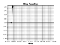
To find the step response of an RC circuit in S multiply the step function in S tines the S function. This is convolution in the frequency domain. Voltage steps are used in testing physical systems.
A unit step is 1/s, a delayed step is (-t*s)/s.
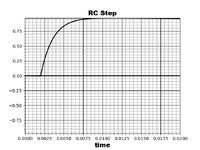
So the step response is( 1/s)*(Src+1). The inverse transform is the tine domain response. 1 - e^(-t/rc)
The inverse FFT is on e way to do the inverse. There wasn’t much on it so I worked out a solution.
In sampled systems. The time and frequency domains are linked by the sampling frequency.
dt = 1/fsample and df = fsample/n
The FFT takes a sampled time domkain signals and creates a complex frequency spectrum. The inverse FFT takes a sampled frequency spectrum and creates a time domain signal.
The function in S is sampled in frequency.
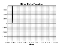
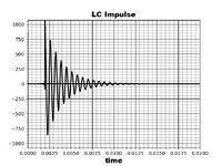
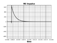
The code takes the inverse FFT of step and impulse responses for a resonant LC circuit and an RC circuit. A theoretical impulse or delta function has an infinite amplitude and frequency content.
The resistors in the LC circuit represent losses.
Mathematically convolving an impulse with a resonant function is like tapping a bell with a hammer.
The impulse response of the LC circuit is a decaying sine wave. 2nd order systems have two forms of energy storage. Energy goes back and forth between the electric field in the capacitor and magnetic field in the inductor, losing energy in each cycle.
The impulse response is used in phsycal testng. There are impulse hammers with force sensors to test mechacal systems. It all has real world usage.
Put a mass on a vertical spring, depress it and let it go. A plot of position versus time about the rest position wil look like the LC response. Energy goes back and forth between the spring and gravitational potential energy.
Systems of the same order have the same forms of responses. Electrical, mechanical, quantum, or biological.
The impulse response of the RC circuit is a decaying exponential. Energy is dumped into the system by the impulse and it dissipates over time. The curve for the RC step response shws the transient solution, a rising exponential, and the steady state solution a constant.
The ringing on the step function is Gibb’s Phenomena, a result of a finite Fourier series.
The forward FFT creates a mirror spectrum. To make it work the S function has to be cooed into the upper half of spectrum array.
Last edited:

