• Welcome to the new Internet Infidels Discussion Board, formerly Talk Freethought.

Practical Math

steve_bank

Diabetic retinopathy and poor eyesight. Typos ...
Joined
Nov 9, 2017
Messages
13,834
Location
seattle
Basic Beliefs
secular-skeptic
A thread for real world applications.

Anything I post will be in Scilab. It is free and an easy install.
 
When dealing with data sets a histogram can be raggedy and hard to make use of. The cumulative distribution is essentially an integration which sooths out the curve.

The majority of the times the cumulative distribution from the data showed a recognizable distribution.

The technique is related to median ranks. The assumption tis that the arithmetic mean represents a 50% balance point, equal weight above and below regardless of distribution.

When you plot sorted data for any distribution the arithmetic mean will align with the 50% point.

You can go through the distributions and vary parameters. Easy entry into probability and statistics.

Open i scilab text editor and copy. Execute from the text editor by clicking on save and execute. Tw plotd will appear, a histogram and cumulative distribution of the data.

// deternines the cumulative distribution for a dara set
// 1 generate radom array
// 2 sort ascending
// 3 calculate pervent up to nth dta point
clear // clears all variables scilab
n =500

// scilab grand(rows, cols, "type", dist parametrs )
p = grand(n, 1, "nor", 70, 3) // normal mean,std
//p = grand(n, 1, "exp", 100 ) // exponential mean
//p = grand(n, 1, "unf", 10, 12) // uniform floats min,max
//p = grand(n, 1, "poi", 100) // poisson mean
//p = grand(n, 1, "uin", 10, 100) // uniform integers min.max

// find average
u = 0
for (h = 1:n)u = u + p(h);end;
av = u/n

sf = 1 // swap flag, 0 no swaps
l = 0 // loop count

// assending bubble sort
// end when no exchages occur
while(sf == 1)
l = l + 1
sf = 0
for(i = 1:n-1)
if (p(i)> p(i+1)) then
temp = p(i)
p(i) = p(i+1)
p(i+1) = temp
sf = 1
end //if

end //for

// runaway loop detector
if( l == n + 500)break;end;

end //while

// percent vs nth data point
// y axis for the cumm dist plot
for( i = 1:n)pc(i) = (i/n)*100;end;

//open plot widows scilab functions
hg = scf(1)
cd=scf(2)
clf(hg)
clf(cd)
scf(hg)
histplot(100,p)
scf(cd)
plot2d(p,pc)
 
https://en.wikipedia.org/wiki/Root_mean_square

The RMS value of a waveform is fundamental in electric circuits. RMS stands for Root Mean Square,i n statistics it is the standard deviation.

The problem with comparing energy content in waveforms is that some can have a DC value of zero, like a sine wave.

Put a resistor in some water. Put a current waveform with a DC average through the resistor and the temperature of the water will rise. Put a different current waveorm with the sane DC average through the resistor and the temperature rise may not be the same.

Current waveforms through the resonator with the same RMS values will result in the same temperature rise.

RMS values represent equivalent heat energy.

RMS f(x)dx = sqrt( (1/(a-b) * integral a,b (f(x)^2))

The integration is usually done numerically on sampled data.

Subtract each data point from the average, square to make all deviations positive, sum, divide by n, take square root.

From a table of integrals integral sin^ 2 = (a/2 -sin(a)/4) – (b/2 – sin(b)/4)

Evaluated between 0 and 2*pi = 0.707

Sine with zero dc is 0.707 * peak voltage
A 50% duty cycle square wave is 0.707


RMS values add root sum square.

The RMS value of an ac waveform with a non zero dc average = sqrt(ac_rms^2 + dc_avg^2)

clear

function [_avg,rms] = avg_rms(x)
[a,b] = size(x)
if(a == 1) then n = b;else n = a;end
_sum = 0
for i = 1:n _sum = _sum + x(i);end;
_avg = _sum/n
_sum = 0
for i = 1: n _sum = _sum + (_avg - x(i))^2;end
_rms = sqrt(_sum/n)
rms = sqrt(_rms^2 + _avg^2)
endfunction

dt = 1e-3
t = [0:dt:1]
n = 10000
for i = 1:n // rectangular wave
ysqw(i) = 0.
if(i <= n/2) ysqw(i) = 1.;end;
end
ysqw = ysqw + 0 // rect wave dc ofset

yramp = t // linear ramp wave
ys = 1 * sin(2*%pi*t) + 0
yn = grand(10000,1,"nor",0,5)
[avg1,rms1] = avg_rms(yn)
// direct sine integration
hil = 2*%pi
lol = 0.
sint = (hil/2 - sin(hil)/4) - (lol/2 - sin(lol)/4)
rmsint = sqrt(sint/hil)

disp(avg1,rms1)
//clf()
//plot2d(ysqw)

Are we having fun yet?
 
Here's another application of "energy" in discrete signal processing. I became acquainted with "energy compaction" in connection with compression methods like JPEG. As in Steve's writing, the energy of a tuple is the root of the sum of squares. I've left out the M (mean) of RMS but that won't matter if you're consistent.

An orthogonal transform will leave a tuple's energy content unchanged — this is a corollary of the Pythagorean Theorem. For example, an orthogonal transform which isolates all DC energy will transform [1 1 1 1] to [2 0 0 0]. Since √(12+12+12+12) = √(22) = √4 = 2, energy is seen to be conserved.

But the cost to encode a coefficient (into a compressed file) is proportional to the energy's logarithm, not to the energy itself. This is the fundamental idea which makes transforms like the DCT which JPEG uses effective for data compression. (The Karhunen-Loeve Transform of an autocorrelation matrix will minimize the sum of these logarithms over random signals described by that autocorrelation.)
 
https://en.wikipedia.org/wiki/Laplace_transform
https://tutorial.math.lamar.edu/classes/de/laplace_table.aspx
https://en.wikipedia.org/wiki/List_of_Laplace_transforms


Under applied math both La Place and Fourier Transforms have equal importance.

La Place Transforms operate in the complex S domain, where S iss the complex variable S = i*2*pi*f.

They are commonly used in the analysis and design of systems and circuits which are dynamic and have a frequency response. Both an electrical series RC circuit and a simple mechanical dash pot damer are singe pile low pass functions.

A pole or zero is of the form (S*tau + 1). Pes are in the denominator and zeros are in the numerator.

The general form is (S*z1 + 1)*(S*z2 + 1).../(S*p1 + 1)*(S*p2 + 1)... which leads to a ratio of polynomials in S.

A single pole or zero represents simple first order differential equation which a has the general solution of Ae^kt. The pole or zero is the tine constant in an eaponetial.

For a simple rc circuit the tine constant is tau = r*c.
For an rc low low pass filter with outpou across the capacitor.
voout = vin * I/(2*pi*f*c)/(r + I/(2*pi*f*c))
dividing through
vout = vin * 1/(i*2*pi*f*r*c +1)
vout/vin = 1/(S*r*c + 1)

The general form of a single pole is 1/(S*TAU + 1) wher TAU is the the time constant. The solution to a first order differential equation is an exponential transient response. e^(t/TAU). It could be an electrical circuit or a simple mechanical dash pot damper.

To derive the time domain solution and solve the differential equation we take the inverse Fourier transform of the S domain function.
S/ frequency domain convolution is multiplication of functions in S. Convincing a sine wave with a single poll RC filter is

omega/((S(i)^2 + omega^2)) * 1/(SRC + 1)

To find the time domain s0lution take the inverse Fourier transform. That is a solution to the time domain differential equation

Vin(t) = i(t) *R + integral(i(t)*dt/C).

There is a saying, 'convolution in the time domain is multiplication in the frequency domain. Putting a time domain sine wave into an rc fillter is time domain convolution.

In the S domain we multiply the LaPlace transform of a sine wave with the transfer function in S. Then take FFT^-1 to gt the time domain output of the filter.

Before PCs there were books of nothing but LaPlace transform pairs. You tried to find a match for a function you were dealing with.

Tools like Scilab and Matlab have automated functions for f(S). Submit a polynomial in S to a function and it returns frequency response, pjase response, and transient response.


clear
R = .01
C = 1000e-6
fres = 1
L = ( 1/(2*%pi*fres*sqrt(C)) )^2
fsin = 100
omega = 2*%pi*fsin
fpole1 = 10
fpole2 = 50
tau1 = 1/(2*%pi*fpole1)
tau2 = 1/(2*%pi*fpole2)
df = .1
freq = .01
fmax = 10000
n = fmax/df
dt = (1/fres)/410
_time = 0
//S domain stmulus signals
for i = 1:n
t(i) = _time
f(i) = freq
S(i) = %i*2*%pi*f(i)
_sin(i) = omega/((S(i)^2 + omega^2))
_ramp(i) = 1/(S(i)^2)
_imp(i) = %e^(-6*S(i))
freq = freq + df
_step(i) = (%e^(-.5*S(i)))/S(i)
_time = _time + dt
end
sintd = fft(_sin,-1)
// S domain filter transfer functions
for i = 1:n
// low pass
y(i) = _sin(i)/(S(i)*tau1 + 1)
// high pass
//y(i) = _sin(i) *(S(i)*tau2)/(S(i)*tau2 + 1)
// band pass
//y(i) = (S(i)*tau1)/(S(i)*tau1 + 1) * 1/(S(i)*tau2 + 1)
// resoant LC tank
y(i) = ( (S(i)*L + R)/(R + S(i)*C)) / ( (R + S(i)*L) + (R + 1/(S(i)*C)) )
magy(i) = abs(y(i))
dbmagy(i) = 20*log10(magy(i))
phasey(i) = atand(imag(y(i))/real(y(i)))
end;
yinv = fft(y,-1)
yinvm = abs(yinv)

Adding: EE Circuits 101 recuew....
 
S(i) is an array of discrete complex frequencies.
y(i) = 1/(S(i)*TAU1 + 1) is a frequency sweep of the circuit.

A plot of the frequency and phase response is called a Bode Plot, pronounced Bow-D. He was a mathematician at Bell during WWII and did a lot of the early work on control systems.

Amplitude is displayed in decibels or db. Decibels are used because serial gains multiply. It is easier to add logs than doing decimal multiplication in your head.

Gain/phase of 1/(S*TAU + 1). A sible pole is caled an integrator. As the input frequency increases the phase shift goes to 90deg,

slpgain.png

slphase.png
 
Combine a low pass function with a high pass function and you get a band pass filter

y(i) = (S(i)*tau1)/(S(i)*tau1 + 1) * 1/(S(i)*tau2 + 1)

sbpgain.png
 
The impulse is an important matemtical construct. An actual impulse does not exist. The theortical impulse has infinite amplitude and zero width. The frequnct trasform of the impule has all frequbces, so convolving te impukse with an S daomain function vealuates it at all frequncies. Hence the transform of the impule response is the frequency response.

t is a time delay. The impulse can be shifted in time.in time.
The impulse %e^(-6*S(i)) has he trnsform

simpulse.png
 
RLC circuit y(i) = ( (S(i)*L + R)/(R + S(i)*C)) / ( (R + S(i)*L) + (R + 1/(S(i)*C)) )..second order, it has poles and zeroes, two forms of energy storage.

First the frequency response which shows a narrow pass band.

Second is the impulse response. Take a ruler and hold one down on the edge f a table with your hand. Flick the end of ruler with a finger and the ruler starts moving. Plot the position of the end of ruler versus time and you will get a sine wave at the resonant frequency of the ruler. That is analogous to the impulse response of a circuit. The motion decays due to losses in the ruler.

A mathematical impulse does the same thing to a resonant parallel RLC circuit. It rings at the resonant frequency for the circuit decaying due to resistance. A damped sine response. The envelope of the decay is a negative exponential determined by the time constant of the circuit. A differential equation has a transient response and a steady state response.

There are criteria to access whether a model can actually be implemented in physical reality. One criteria is that the area under the impulse reponse curve must be finite. That is an expression of the Laws Of Thermodynamics.

If the circuit is simulated without resistance it will oscillate forever, the area under the impulse response curve is not finite as t->inf over time.

slcmag.png

simpresp.png

simpresp2.png

No resitance response -- impossible to achieve
 
The flip side to S-frequency domain is ti me domain convolution.


The first plot shows the sine wave response >> the cuttof frequency or pole of the low pass function. A first order low pass acts like an integrator, meaning there is a 90deg phase shift. Integrating sine yields cosine.

The next plots show the impulse response. The Fourier transform of the impulse response yields the frequency response. This is not imited to electric circuits.

https://en.wikipedia.org/wiki/Modal_testing
An ideal impact to a structure is a perfect impulse, which has an infinitely small duration, causing a constant amplitude in the frequency domain; this would result in all modes of vibration being excited with equal energy. The impact hammer test is designed to replicate this; however, in reality a hammer strike cannot last for an infinitely small duration, but has a known contact time. The duration of the contact time directly influences the frequency content of the force, with a larger contact time causing a smaller range of bandwidth. A load cell is attached to the end of the hammer to record the force. Impact hammer testing is ideal for small light weight structures; however as the size of the structure increases issues can occur due to a poor signal to noise ratio. This is common on large civil engineering structures.


In mechanics it is called modal analysis, modes being resonances. Eigem values and Eigen vectors of the system function.

Imagine the open steel frame of a building. Hit it with a short force pulse and measure the response at nodes in the structure. The transformation of the impulse repose yields the resonances of the structure. Like striking a bell. You can find impact or impulse hammers online that measure the force and duration of hitting a structure.

Tesla was alleged to have shaken a building by exciting a resonance ,

Quantum mechanics, Newtonian mechanics, electric circuits all are the same basic principles, but with different names.
 
A simple first order differential equation.

The continuity equation for a simple series resistor capacitor circuit driven by a voltage is

Vr voltage across the resistor
Vc voltage across te capacitor

Vvin – Vr – Vc = 0

Conservation, at any time all voltages must sum to zero

The differential equation for a capacitor is I = c*dv/dt,
Solving for the capacitor voltage dv = (i/c)* dt.
For a constant current using Euler's Method,

Vcap = 0 // initial conditions
for I = 1:n Vcap = Vcap + (I/C)*dt);end;

Vin(t) - (i(t) *r) +- (integral((i(t)/C) dt) = 0
vin(t) = (i(t) *r) + (integral((i(t)/C) dt)
Calculate the current at time t, estimate the change in capacitor voltage, recalculate current...

Euler's Method


clear

//sine, square, and impulse waves
function [y] = makewave(j,f,t,a)
[d,nt] = size(t)
if j == 1 then
for k = 1:nt
y(k) = 0
if(k > floor(nt/4)) y(k) = a;end;
end
end
if(j == 2) y = a * sin(2*%pi*f.*t);end;
if(j == 3) then
for i = 1:nt y(i) = 0;end;
y(floor(nt/4)) = a
end
endfunction

_sin = 2
step = 1
imp = 3

// given r and the 3db pole frequency of the circuit calculate required cap
fp = 5 // 3db frequency
r = 1000
c = 1/(2*%pi*fp*r)
fc = 1/(2*%pi*c*r)

dt = .001
t = [0:dt:.5] // time record
[d,nt] = size(t)
f = 5 // sine frequency
amp = 1
y1 = makewave(_sin,f,t,5)

vc = 0 // initial condition
for j = 1:nt
vr = y1(j) - vc
_i(j)= vr/r
dvc = (_i(j) * dt)/c
vc = vc + dvc
vout(j) = vc
end
plot(vout)
 
timer.png

sin input and filtered reduced amplitude output
 
impt.png

Input impulse

impr.png

Impulse response

fr.png

Transform of the impulse response, frequency response.
 
On to the discrete time. Digital filetrs come under the heading of Digital Signal Processing. Low cost fast processors have rplaced a lot of analiog continuous time processing. It starts with sampling.


https://en.wikipedia.org/wiki/Nyquist–Shannon_sampling_theorem

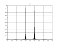
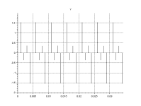
The Nyquist–Shannon sampling theorem is a theorem in the field of signal processing which serves as a fundamental bridge between continuous-time signals and discrete-time signals. It establishes a sufficient condition for a sample rate that permits a discrete sequence of samples to capture all the information from a continuous-time signal of finite bandwidth.

Strictly speaking, the theorem only applies to a class of mathematical functions having a Fourier transform that is zero outside of a finite region of frequencies. Intuitively we expect that when one reduces a continuous function to a discrete sequence and interpolates back to a continuous function, the fidelity of the result depends on the density (or sample rate) of the original samples. The sampling theorem introduces the concept of a sample rate that is sufficient for perfect fidelity for the class of functions that are band-limited to a given bandwidth, such that no actual information is lost in the sampling process. It expresses the sufficient sample rate in terms of the bandwidth for the class of functions. The theorem also leads to a formula for perfectly reconstructing the original continuous-time function from the samples.

If you run the code and vary fsig in increments of the sampling frequency, the result will be the same. 10Hz, fs+ 10hz, 2fs + 10hz… will all look the same, 10hz..

When the signal is > fs/2, the Nyquist frequency, aliasing occurs. For fs = 1000hz a signal of 520 hz aliases to fs/2 - 20hz

The FFT has a mirror spectrum shown in the first plot. We only need to show half. The spectrum is centered at fs/2.

The plot shows a 10 hz signal sampled at 1000 hz, If I change fsig to 1010, the result will still be 10 hz. This is born out by the FFT.

Intentional under sampling and aliasing is actually used as a technique to shift frequencies.

Clear
fs = 1000 // sampling frequency Hz
dt = 1/fs // sampling interval seconds
t = [0:dt:1] // time base 1 second
n = length(t)
df = fs/n // frequency resolution
f = [0:df:fs – df] // frequency scaling for the FFT plot
fsig1 = 200 //signal frequency
fsig2 = 700
y1 = sin(2*%pi*fsig1*t)
y2 = sin(2*%pi*fsig2*t)
y = y1 + y2
yf = fft(y,1)
yfmag = 2*abs(yf)

w1 = scf(1)
clf(w1)
plot2d3( f(1:n/2),yfmag(1:n/2) )
title("MAG")
gca().grid=[1 1 1 ]
w2 = scf(2)
clf(w2)
plot2d(t,y)
title("Y")
gca().grid=[1 1 1]
 
[alfftfull.png

Full FFT plot. Mirror images about fs/2 sin1 + sin2
 

Attachments

  • als2sigalias.png
    als2sigalias.png
    7.3 KB · Views: 1
als2sigalias.png

sin1 20 hz + sin2 700hz. 200hz shows correctly, 700hz aliased to 300hz.
 

Attachments

  • alsam.png
    alsam.png
    6.8 KB · Views: 1
Back
Top Bottom