steve_bank
Diabetic retinopathy and poor eyesight. Typos ...
One of the first feedback control mechanisms applied to dynamic systems may be the centrifugal speed regulator for a steam engine. Mathematically there is no difference between that and a power supply or a cruise control on a car.
In electronics an early problem was stabilizing gain of tube amplifiers in long distance telephone lines. When the amp is palced inside a feedback loop the audio out is compared to the output and the error amplifier adjusts the input to audio amp as gain changes.
At Bell Labs during WWII modern control theory was developed. A mathematician Bode was a major contributor. I read his book,
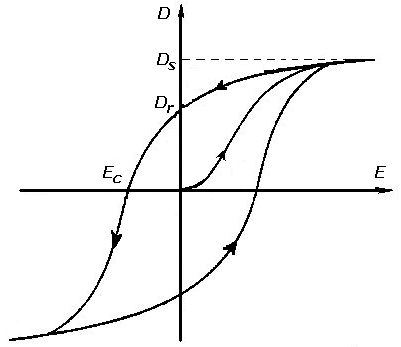
Tubes and transistors vary with temperature, voltages, and from part to part. They are also non linear. Feedback loops linearize the system reducing distortions. Audiophiles argue that feedback actual adds distortion which is true, but the distortion is below hearing threshold.
Pro[ortional control is straightforward. You press the gas petal on a car proportional to the diffence between the trarget speed and current speed. In this case your brain is the controller, your leg/foot is the proportional output of the controller to the plant which is the engine.
There are three general modes of response
Critical damping is when you transition to the target speed as quickly as possible without any overshoot.
Over damped is when you approach the target speed slowly with no overshoot.
Under damped is when you go petal to the metal , overshoot and back off the gas, then hit it again going above and below the target until you settle on the target speed.
The choice of damping depends on what you need. You may want fast response time and live with overshoot. Sometimes overshoot can be harmful. It all depnds.
A PID temperature controller.
The proportional term determines steady state acxurcay and load regulation, and affects trasient response.The derivative term responds to the shot term rate of change. The integral term responds to long term trends. Theoretically the integral term reduces error to zero, but that is impossible. If the output is exactly equal to the input the error goes to zero and there is no signal to drive the plant in this case a heater.
kp is proportional gain. Fb is the feedback, if the output is directly compared to the input the feedback is 1.
Stability analysis is done in the frequency, complex S La Place, domain using techniques like Bode plots and root locus.
 en.wikipedia.org
https://en.wikipedia.org/wiki/Barkhausen_stability_criterion
The Barkhausen Criteria says that in a general linearr system it will oscillate when the loop gain is 1 and the phase shift around the loop is 360 degrees.
For a system to physically realizable and stable the impulse response must go to zero as time goes to infinity. It means if you thunp a bell, convolving an impulse with the bell, it will ring and decay as time passes. It will not ring forever. A system can be mathematically constructed and simulated that can not be physically implemented.
The Bode Plot plots he open loop gain and phase and is useds to asses stability. The forward gain is the ‘plant’ and the load. The fedback gain is from the load to te controller. The loop gain is Aforward(S) * Afeedback(). The two functions reduce to polynomials in S. The factors of the polynomials are the system poles and zeros and are piloted as root locus.
Stability is based on the frequency response of the open loop gain. When the phase shift is multiples of 360 degrees at a frequency with sufficient gain at the frequncy the system becomes an oscillator. Stability compensation involves modifying the open loop gain frequency response.
https://en.wikipedia.org/wiki/PID
The code is a parallel PID controller. It has a analog electronic form.
Kuo is an old text but good if you are interested.
The thermal model is calculating the change in temperature by q = m*c*dT. The loos terms rpresent system entropy. The loss terms are not eaxactly correct but serve to make the model realistic.
The code was run on Codeblocks. You can tnker with it.
Real systems have voltage limits, when a clayclted voltage eceds a limit it is kinited to the max voltage,
Rtherm rrpesents the thermal resitance from the load to ambient. You can vary heater resistance, volage maximum, and Rtherm.
To see he time response you will have to plot results. I use Scilab, it can be done in a spreadsheet.
For a setpoint of 50 and an ambient of 27. Keep in mind 6 decimal places in maost applcations is meningless.
kp = 100, kd = 0, ki = 0 temperature is 48.100797
kp = 100, kd = 0, ki = 300 temperature = 49. 504950
The integral works as advertised.
Kp = 1000, kd = 0, ki = 0 temperature = 49.90969
Proportional alone can work. Integral comes into play when there are losses and other systemic errors in the sytem. Raising proprtional gain has limits and can lead to stability problems.
dt sets the resolution. If it is too big it won’t work properly.
void save(int n, double *x, double *y) {
int i;
ofstream sigfile;
sigfile.open("sig.txt");
sigfile << n << "\n";
for (i = 0; i < n; i++)
sigfile << x << " " << y<< "\n";
sigfile.close();
cout << "SAVE DONE" << "\n";
}//save()
double integral(int n,double *x, double delt){
// simple rectangular integration
double y = 0;
for(int i = 0; i < n; i++)y = y + x * delt;
return") ;
;
}//integral()
double Rloss = 65000, dTloss = 0,qloss = 0;
double Cp = .4, load_temp = 0,Tamb = 27, load_mass = 1;
double kp = 0, kd = 0, ki = 0;
double Verror = 0, dt = .00001, Tsetpoint = 50, Vmax = 200;
double prop = 0,deriv = 0, integ = 0,Vplant = 0;
double Rheater = 1, q = 0, heater_power = 0;
double heater_efficency = 0.9, _time = 0, dT = 0;
double Tmax = 0,sim_time = 3;
int i = 0, j = 0, N = 0, Nbuf = 1000;
int main(){
N = int(sim_time/dt); //record length
double *buf = new double[Nbuf];
double *Tload = new double[N];
double *t = new double[N];
load_temp = Tamb;
for(i = 0; i < Nbuf;i++)buf = 0;
kp = 1e6; kd = 0; ki = 0;
for( i = 0; i < N; i++) {
t = _time;// time base
_time += dt;
//push load temperature onto the buffer
for(j = 1; j < Nbuf;j++)buf[j - 1] = buf[j];
buf[Nbuf-1] = load_temp;
Verror = Tsetpoint - load_temp;
if(Verror < 0) Verror = 0; // check for power supply saturation
if(Verror > Vmax) Verror = Vmax;
prop = kp * Verror;
deriv = kd * (buf[Nbuf-1] - buf[Nbuf-2])/dt;
integ = ki * integral(Nbuf,buf,dt);
Vplant = prop + deriv + integ;
if(Vplant < 0) Vplant = 0;
if(Vplant > Vmax) Vplant = Vmax;
heater_power = pow(Vplant,2)/Rheater; // watts
q = heater_efficency * heater_power * dt/1000.; // kilo joules
dT = q/(load_mass * Cp);
qloss = (load_temp - Tamb)/Rloss;
dTloss = qloss/(load_mass * Cp);
load_temp +=(dT - dTloss);
Tload = load_temp;
} //for
save(N, t, Tload);
Tmax = Tload[N-1];
printf("N %d \n",N);
printf("Steady State %f \n",Tmax);
}//min()
In electronics an early problem was stabilizing gain of tube amplifiers in long distance telephone lines. When the amp is palced inside a feedback loop the audio out is compared to the output and the error amplifier adjusts the input to audio amp as gain changes.
At Bell Labs during WWII modern control theory was developed. A mathematician Bode was a major contributor. I read his book,
Tubes and transistors vary with temperature, voltages, and from part to part. They are also non linear. Feedback loops linearize the system reducing distortions. Audiophiles argue that feedback actual adds distortion which is true, but the distortion is below hearing threshold.
Pro[ortional control is straightforward. You press the gas petal on a car proportional to the diffence between the trarget speed and current speed. In this case your brain is the controller, your leg/foot is the proportional output of the controller to the plant which is the engine.
There are three general modes of response
Critical damping is when you transition to the target speed as quickly as possible without any overshoot.
Over damped is when you approach the target speed slowly with no overshoot.
Under damped is when you go petal to the metal , overshoot and back off the gas, then hit it again going above and below the target until you settle on the target speed.
The choice of damping depends on what you need. You may want fast response time and live with overshoot. Sometimes overshoot can be harmful. It all depnds.
A PID temperature controller.
The proportional term determines steady state acxurcay and load regulation, and affects trasient response.The derivative term responds to the shot term rate of change. The integral term responds to long term trends. Theoretically the integral term reduces error to zero, but that is impossible. If the output is exactly equal to the input the error goes to zero and there is no signal to drive the plant in this case a heater.
kp is proportional gain. Fb is the feedback, if the output is directly compared to the input the feedback is 1.
Stability analysis is done in the frequency, complex S La Place, domain using techniques like Bode plots and root locus.
Root locus analysis - Wikipedia
Definition. The root locus of a feedback system is the graphical representation in the complex s-plane of the possible locations of its closed-loop poles for varying values of a certain system parameter. The points that are part of the root locus satisfy the angle condition.
https://en.wikipedia.org/wiki/Barkhausen_stability_criterion
The Barkhausen Criteria says that in a general linearr system it will oscillate when the loop gain is 1 and the phase shift around the loop is 360 degrees.
For a system to physically realizable and stable the impulse response must go to zero as time goes to infinity. It means if you thunp a bell, convolving an impulse with the bell, it will ring and decay as time passes. It will not ring forever. A system can be mathematically constructed and simulated that can not be physically implemented.
The Bode Plot plots he open loop gain and phase and is useds to asses stability. The forward gain is the ‘plant’ and the load. The fedback gain is from the load to te controller. The loop gain is Aforward(S) * Afeedback(). The two functions reduce to polynomials in S. The factors of the polynomials are the system poles and zeros and are piloted as root locus.
Stability is based on the frequency response of the open loop gain. When the phase shift is multiples of 360 degrees at a frequency with sufficient gain at the frequncy the system becomes an oscillator. Stability compensation involves modifying the open loop gain frequency response.
https://en.wikipedia.org/wiki/PID
The code is a parallel PID controller. It has a analog electronic form.
Kuo is an old text but good if you are interested.
The thermal model is calculating the change in temperature by q = m*c*dT. The loos terms rpresent system entropy. The loss terms are not eaxactly correct but serve to make the model realistic.
The code was run on Codeblocks. You can tnker with it.
Real systems have voltage limits, when a clayclted voltage eceds a limit it is kinited to the max voltage,
Rtherm rrpesents the thermal resitance from the load to ambient. You can vary heater resistance, volage maximum, and Rtherm.
To see he time response you will have to plot results. I use Scilab, it can be done in a spreadsheet.
For a setpoint of 50 and an ambient of 27. Keep in mind 6 decimal places in maost applcations is meningless.
kp = 100, kd = 0, ki = 0 temperature is 48.100797
kp = 100, kd = 0, ki = 300 temperature = 49. 504950
The integral works as advertised.
Kp = 1000, kd = 0, ki = 0 temperature = 49.90969
Proportional alone can work. Integral comes into play when there are losses and other systemic errors in the sytem. Raising proprtional gain has limits and can lead to stability problems.
dt sets the resolution. If it is too big it won’t work properly.
void save(int n, double *x, double *y) {
int i;
ofstream sigfile;
sigfile.open("sig.txt");
sigfile << n << "\n";
for (i = 0; i < n; i++)
sigfile << x << " " << y<< "\n";
sigfile.close();
cout << "SAVE DONE" << "\n";
}//save()
double integral(int n,double *x, double delt){
// simple rectangular integration
double y = 0;
for(int i = 0; i < n; i++)y = y + x * delt;
return
;}//integral()
double Rloss = 65000, dTloss = 0,qloss = 0;
double Cp = .4, load_temp = 0,Tamb = 27, load_mass = 1;
double kp = 0, kd = 0, ki = 0;
double Verror = 0, dt = .00001, Tsetpoint = 50, Vmax = 200;
double prop = 0,deriv = 0, integ = 0,Vplant = 0;
double Rheater = 1, q = 0, heater_power = 0;
double heater_efficency = 0.9, _time = 0, dT = 0;
double Tmax = 0,sim_time = 3;
int i = 0, j = 0, N = 0, Nbuf = 1000;
int main(){
N = int(sim_time/dt); //record length
double *buf = new double[Nbuf];
double *Tload = new double[N];
double *t = new double[N];
load_temp = Tamb;
for(i = 0; i < Nbuf;i++)buf = 0;
kp = 1e6; kd = 0; ki = 0;
for( i = 0; i < N; i++) {
t = _time;// time base
_time += dt;
//push load temperature onto the buffer
for(j = 1; j < Nbuf;j++)buf[j - 1] = buf[j];
buf[Nbuf-1] = load_temp;
Verror = Tsetpoint - load_temp;
if(Verror < 0) Verror = 0; // check for power supply saturation
if(Verror > Vmax) Verror = Vmax;
prop = kp * Verror;
deriv = kd * (buf[Nbuf-1] - buf[Nbuf-2])/dt;
integ = ki * integral(Nbuf,buf,dt);
Vplant = prop + deriv + integ;
if(Vplant < 0) Vplant = 0;
if(Vplant > Vmax) Vplant = Vmax;
heater_power = pow(Vplant,2)/Rheater; // watts
q = heater_efficency * heater_power * dt/1000.; // kilo joules
dT = q/(load_mass * Cp);
qloss = (load_temp - Tamb)/Rloss;
dTloss = qloss/(load_mass * Cp);
load_temp +=(dT - dTloss);
Tload = load_temp;
} //for
save(N, t, Tload);
Tmax = Tload[N-1];
printf("N %d \n",N);
printf("Steady State %f \n",Tmax);
}//min()
Last edited: