• Welcome to the new Internet Infidels Discussion Board, formerly Talk Freethought.

Interpolation And Curve Fitting

steve_bank

Diabetic retinopathy and poor eyesight. Typos ...
Joined
Nov 9, 2017
Messages
13,769
Location
seattle
Basic Beliefs
secular-skeptic
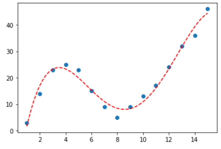
Lagrange interpretation is easy. Before PCs on everybody's desk I coded it in a programmable calculator to interpolate tables.

In the early days of slow embedded processors interpolation of trig function precalculated tables s could be faster than other means.

You can change he curve and number of points to experiment with it.


Code:
# Python
import math

def lagrange(x,xd,yd):
    n = len(xd)
    y = 0
    for i in range (n):
        wp = yd[i]
        for j in range(n):
            if j != i:
                wp = wp * (x - xd[j])/(xd[i] - xd[j])
        y += wp
    return y

n = 7
xd = n*[0]
yd = n*[0]
lo = 0
hi = math.pi/2  # x range 0 to 90 degrees
dx = (hi-lo)/(n-1)

#ceate data table
for i in range(n):
    xd[i] = dx * i
    yd[i] = math.sin(xd[i])
                
xrad = math.pi/7  #x value to be interpolated
xdeg = xrad*180/math.pi
ya = math.sin(xrad) #actual value
y = lagrange(xrad,xd,yd)
print('angle rad-deg    ',xrad,'   ',xdeg)
print('sim actua-interp   ',ya,'   ',y)
 
Lagrange's formula, while theoretically correct, isn't the best computationally, from cancellation and from computational efficiency.

A mathemtically-equivalent alternative is  Newton polynomial also Newton's Divided Difference Interpolation Formula -- from Wolfram MathWorld One can do some precalculation for it with  Divided differences also Divided Difference -- from Wolfram MathWorld so one can more quickly do interpolation repeatedly. Divided differences also have good cancellation properties.

Another mathemtically-equivalent alternative is  Neville's algorithm also Neville's Algorithm -- from Wolfram MathWorld calculating a pyramid of intermediate results much like divided differences.
 
Solving linear equations. There are high level functions in Python to do it.

Solving simultaneous equations.

2x + y = 10
x + y = 9

In matrix form
a =
2 1
1 1

b =
10
9

c =
x
y

Algebraically c = a/b but matrix division is not defined, the multiplicative inverse is defined b^-1 or inv(). So c = a^-1 * b.

In Python

import math
import array as ar
import numpy as np
from numpy.linalg import inv

a = np.array([[2,1],[1,1]], np.float64)
b = np.array([[10],[9]], np.float64)
print(b)
print(a)
xy = np.matmul(inv(a),b)

print(xy) -- the solution x = 1, y = 8

To fit a polynomial to a data set the equations have to be synthesized to solve for the polynomial coefficients.

Numpy needs to be installed, the ndarray function makes it easier.

You can vary ndata and see the results, and create different data sets and see what happens. Depending on the data and degree polynomials can oscillate between data points.

A 5th order is a close approbation to a library sin. You could compare execution time for the compiled c sin() and a polynomial approximation assuming the coefficients have been precalculated.

Code:
mport math as ma
import array as ar
import numpy as np
from numpy.linalg import inv
import matplotlib.pyplot as plt


def poly_eval(coef,x):
    s = 0
    rows,cols = np.shape(coef)
    n = rows-1
    for i in range(rows):
        s += pow(x,n)*coef[i]
        n -= 1
    return s

def poly_coef(data):
    # linear equati solver
    # generate polynomial coeficients
    # c = b/a . a = n equations in n unowns square matrix
    [rows,cols] = np.shape(data)
    b = np.ndarray(shape = (rows,1))
    a = np.ndarray(shape=(rows,rows))
    for i in range(rows): b[i][0] = data[i][cols-1]
    for r in range(rows):
        n = rows - 1
        for c in range(rows):   
            a[r][c] = pow(data[r][0],n)
            n -= 1
    c = np.matmul(inv(a),b)  # order of matrix multiplicatio matters
    return c

n = 20  # number of inyerpolations
ndata = 6  # number data smaples
xmax = ma.pi*2  # sin() 360 degrees
x= n*[0]
y = n*[0]  # interpolated sin
ys = n*[0] # sin() libray function
data =np.ndarray(shape = (ndata,2))
x = np.linspace(0,xmax,n)  # 3*pi raduans
t = np.linspace(0,xmax,ndata)

# sampled sin()
for i in range(ndata):
    data[i][1] = ma.sin(t[i])
    data[i][0] = t[i]
  
coef = poly_coef(data)

for i in range(n):
    y[i] = poly_eval(coef,x[i])
    ys[i] = ma.sin(x[i])
    print(x[i],"   ",y[i],"   ",ys[i])


[fig, ax] = plt.subplots()
ax.plot(x, y, linewidth=2.0,color='r')
ax.plot(x, ys, linewidth=2.0,color='k')
ax.grid(color='k', linestyle='-', linewidth=2)
plt.show()
 
Determinants? That's Cramer's rule. While it is theoretically correct, it's cumbersome in practice. One should only need to do it if one wants to invert a lot of small matrices very fast. Otherwise, something like Gaussian elimination or LU decomposition or Cholesky decomposition will do it. Those are algorithms for solving systems of linear equations:

A.x = b

What one does to find a matrix inverse is to solve for several b's at once, where those combined b's are the identity matrix.

I once had to invert some matrices analytically in Python and C++ and those matrices' coefficients were integers. So I used a fraction class for the calculation, converting those integers into fractions with denominator 1 before beginning.

Python as a built-in fraction class, and one can easily find one for C++ online. For C++, one would use a template class, where the template type is whatever type of integer you want to use. Worried about overflows? One can use a bignum-integer class, an arbitrary-precision one.
 
Python Numpy has a linear equation solver. From the Nunpy docs Numoy linear algebra uses the LAPAK library which evolved out of LINPAK, both written in FORTRAN.

LINPK was one of the original libraries.

Math packages generally use a common set of math libraries, usually FORTAN legacies.

If I was actually solving a problem I'd use Matlab or Scilab. Th Python Numpy combo is too clumsy. In Scilab all variables are matrices. Arithmetic operators are automatically overloaded making it easier to code.

Numpy curve fitting and linear algebra


Linking and calling LINPAK from C


Coding basic algorithms was how I leaned new math.
 
Using the Numpy builtins to interpolate.

The first code I posed and the Numpy functions give the same results for the same data set.

Code:
import math as ma
import array as ar
import numpy as np
from numpy.linalg import inv
import matplotlib.pyplot as plt
import warnings


def poly_eval(coef,x):
    s = 0
    rows,cols = np.shape(coef)
    n = rows-1
    for i in range(rows):
        s += pow(x,n)*coef[i]
        n -= 1
    return s


n = 20  # number of interpolations
ndata = 7# number data samples
xmax = ma.pi*2  # sin() 360 degrees
#x= n*[0]
x = np.ndarray(shape=(n,1),dtype = np.float64)
y = np.ndarray(shape = (n),dtype = np.float64)  # interpolated sin
ys = np.ndarray(shape = (n),dtype = np.float64) # sin() libray function
yd = np.ndarray(shape = (n),dtype = np.float64)
data = np.ndarray(shape = (ndata),dtype = np.float64)

x = np.linspace(0,xmax,n)  # 2*pi raduans
t = np.linspace(0,xmax,ndata)

# sampled sin()
for i in range(ndata):
    data[i] = ma.sin(t[i])
  
coef = np.polyfit(t, data,ndata-1)

print("x, sin(x), interpolated sin(x)")
for i in range(n):
    y[i] = np.polyval(coef, x[i]) # interpolared sine
    ys[i] = ma.sin(x[i]) # libray sine
    print("%2.8f  %+2.15f   %+2.15f" %(x[i],ys[i],ys[i]))

print("coefficients")
for i in range(len(coef)):
        print(coef[i])


[fig, ax] = plt.subplots()
ax.plot(x, y, linewidth=2.0,color='r')
ax.plot(x, ys, linewidth=2.0,color='k')
ax.grid(color='k', linestyle='-', linewidth=2)
plt.show()


Code:
Results from first code
x, sin(x), interpolated sin(x)
0.00000000f  +0.000000000000000   +0.000000000000000
0.33069396f  +0.324699469204683   +0.324699469204683
0.66138793f  +0.614212712689668   +0.614212712689668
0.99208189f  +0.837166478262529   +0.837166478262529
1.32277585f  +0.969400265939330   +0.969400265939330
1.65346982f  +0.996584493006670   +0.996584493006670
1.98416378f  +0.915773326655058   +0.915773326655058
2.31485774f  +0.735723910673132   +0.735723910673132
2.64555171f  +0.475947393037074   +0.475947393037074
2.97624567f  +0.164594590280734   +0.164594590280734
3.30693964f  -0.164594590280734   -0.164594590280734
3.63763360f  -0.475947393037073   -0.475947393037073
3.96832756f  -0.735723910673131   -0.735723910673131
4.29902153f  -0.915773326655057   -0.915773326655057
4.62971549f  -0.996584493006670   -0.996584493006670
4.96040945f  -0.969400265939330   -0.969400265939330
5.29110342f  -0.837166478262529   -0.837166478262529
5.62179738f  -0.614212712689668   -0.614212712689668
5.95249134f  -0.324699469204684   -0.324699469204684
6.28318531f  -0.000000000000000   -0.000000000000000
[-3.3258563e-17]
[-0.00573068]
[0.09001734]
[-0.40848573]
[0.29614518]
[0.86834301]
[0.]

Numpy functios results
x, sin(x), interpolated sin(x)
0.00000000  +0.000000000000000   +0.000000000000000
0.33069396  +0.324699469204683   +0.324699469204683
0.66138793  +0.614212712689668   +0.614212712689668
0.99208189  +0.837166478262529   +0.837166478262529
1.32277585  +0.969400265939330   +0.969400265939330
1.65346982  +0.996584493006670   +0.996584493006670
1.98416378  +0.915773326655058   +0.915773326655058
2.31485774  +0.735723910673132   +0.735723910673132
2.64555171  +0.475947393037074   +0.475947393037074
2.97624567  +0.164594590280734   +0.164594590280734
3.30693964  -0.164594590280734   -0.164594590280734
3.63763360  -0.475947393037073   -0.475947393037073
3.96832756  -0.735723910673131   -0.735723910673131
4.29902153  -0.915773326655057   -0.915773326655057
4.62971549  -0.996584493006670   -0.996584493006670
4.96040945  -0.969400265939330   -0.969400265939330
5.29110342  -0.837166478262529   -0.837166478262529
5.62179738  -0.614212712689668   -0.614212712689668
5.95249134  -0.324699469204684   -0.324699469204684
6.28318531  -0.000000000000000   -0.000000000000000
coefficients
-5.284354243250287e-17
-0.005730681815105242
0.09001733945198447
-0.40848572890386464
0.2961451765432327
0.8683430102893087
-1.3427995533605042e-15

What method does linalg solve use?
1 Answer. From the numpy docs: solve is a wrapper for the LAPACK routines dgesv and zgesv, the former being used if a is real-valued, the latter if it is complex-valued. The solution to the system of linear equations is computed using an LU decomposition [R40] with partial pivoting and row interchanges.Dec 10, 2012
 
I screwed that one up, I had the print statements wrong. I should have realized it looked too good to be true.

The two methods have similar results but not exactly the same.

Code:
Order 10
Results 1st code posted

0.00000000f  +0.000000000000000   +0.000000000000000
0.33069396f  +0.324699469204683   +0.324642052634832
0.66138793f  +0.614212712689668   +0.614209372737415
0.99208189f  +0.837166478262529   +0.837174599918376
1.32277585f  +0.969400265939330   +0.969401529584253
1.65346982f  +0.996584493006670   +0.996582686217054
1.98416378f  +0.915773326655058   +0.915772822592789
2.31485774f  +0.735723910673132   +0.735724393285762
2.64555171f  +0.475947393037074   +0.475947570790514
2.97624567f  +0.164594590280734   +0.164594525308484
3.30693964f  -0.164594590280734   -0.164594525308483
3.63763360f  -0.475947393037073   -0.475947570790515
3.96832756f  -0.735723910673131   -0.735724393285763
4.29902153f  -0.915773326655057   -0.915772822592790
4.62971549f  -0.996584493006670   -0.996582686217053
4.96040945f  -0.969400265939330   -0.969401529584246
5.29110342f  -0.837166478262529   -0.837174599918360
5.62179738f  -0.614212712689668   -0.614209372737414
5.95249134f  -0.324699469204684   -0.324642052634800
6.28318531f  -0.000000000000000   +0.000000000000003
np poly fit
x, sin(x), interpolated sin(x)
0.00000000  +0.000000000000000   -0.000000000000007
0.33069396  +0.324699469204683   +0.324642052634879
0.66138793  +0.614212712689668   +0.614209372737420
0.99208189  +0.837166478262529   +0.837174599918356
1.32277585  +0.969400265939330   +0.969401529584237
1.65346982  +0.996584493006670   +0.996582686217049
1.98416378  +0.915773326655058   +0.915772822592792
2.31485774  +0.735723910673132   +0.735724393285765
2.64555171  +0.475947393037074   +0.475947570790515
2.97624567  +0.164594590280734   +0.164594525308481
3.30693964  -0.164594590280734   -0.164594525308485
3.63763360  -0.475947393037073   -0.475947570790517
3.96832756  -0.735723910673131   -0.735724393285767
4.29902153  -0.915773326655057   -0.915772822592798
4.62971549  -0.996584493006670   -0.996582686217063
4.96040945  -0.969400265939330   -0.969401529584257
5.29110342  -0.837166478262529   -0.837174599918363
5.62179738  -0.614212712689668   -0.614209372737391
5.95249134  -0.324699469204684   -0.324642052634821
6.28318531  -0.000000000000000   +0.000000000000004
 
Back
Top Bottom