steve_bank
Diabetic retinopathy and poor eyesight. Typos ...

LC circuit - Wikipedia
The Fourier Transform is a link between time and frequency domains. For any time domain function f(t) there is one and only one Fourier Transform F(s) and vice versa. There is a proof I forget the name.
To test a resonant parallel LC circuit I could put a voltage step into the circuit with a signal generator and capture the output on an oscilloscope.
Mathematically it is the time domain convolution of the signal and the circuit time domain differential equations. Scroll down to the convolution integral.
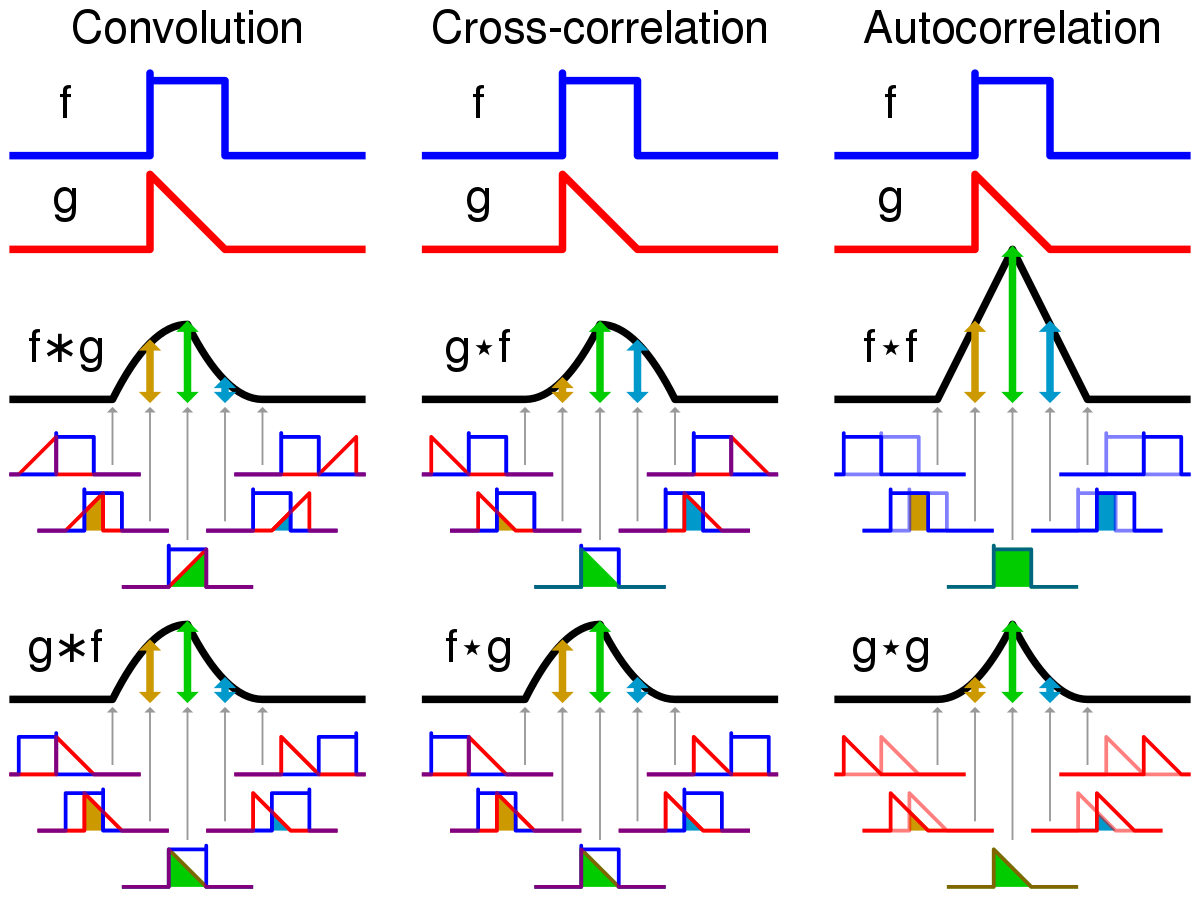
Convolution - Wikipedia
There is a saying 'convolution in the time domain is multiplication in the frequency domain'. To solve a differential equation convert to the frequency(S) domain and take the inverse FFT. Frequency to time.
The Laplace Transform is similar to the Fourier Transform and is used to create time-frequency domain pas. There used to be books of pairs. You looked up a frequency domin function that matched your circuit and read the time domain solution.
The differential equations for a capacitor and induct or are i = C * dv/dt v= L* di/dt. The equations represet energy storage in magnetic and electric fields.
Adding parasitic resistance for the induct or and capacitor the frequency equations are
rc + 1/Sc and rl + Sl where S is the complex frequency variable.
Without resistance the circuit will mathematically violate LOT and oscillate forever.
The LaPlace transform for a 1st order equation is S. Replace the derivatives with S and find the frequency response. Then take the inverse FFT.
The LaPlace transform of a delayed step function is
np.exp(-.5*S)/S.
The LaPlace transform of a parallel LC circuit is
(rl+S*L)*(rc+1./(S*C))/(rl + rc + S*L +1./(S*C))
The frequency domain convolution is
(rl+S*L)*(rc+1./(S*C))/(rl + rc + S*L +1./(S*C)) * np.exp(-.5*S)/S.
Resonant frequency is 1/(2*pi*sqrt(LC), Given resonant frequency and capacitor inductor is calculated.
Take the inverse FFT to get the time domain solution. If you run the code you will see the usual 2nd order exponential transient response and decaying sine wave at the resonant frequency.
The Bode plot is the frequency response of a band pass filter. You can play around with parameters and see the results.
The technique applies to any dynamic system. The LC circuit example is analogous to what could be done with a mechanical bell, a maniacal resonator.
There is beaucoup information on LaPlace trasfrm on the net.
Code:
import numpy as np
import matplotlib.pyplot as plt
#----------------------------------------------------------------
def plotxy(xlo,xhi,ylo,yhi,x,y,title,xlabel,ylabel):
        font1 = {'family': 'arial',
        'color':  'black',
        'weight': 'heavy',
        'size': 15,
        }
        [fig, p1] = plt.subplots(1)
        p1.plot(x,y,linewidth=2.0,color="k")
        p1.grid(color='k', linestyle='-', linewidth=1)
        p1.grid(which='major', color='k',linestyle='-', linewidth=0.8)
        p1.grid(which='minor', color='k', linestyle='-', linewidth=0.3)
        p1.set_xlim(xlo,xhi)
        p1.set_ylim(ylo,yhi)
        p1.set_title(title, fontdict = font1)
        p1.set_xlabel(xlabel, fontdict = font1)
        p1.set_ylabel(ylabel, fontdict = font1)
        p1.minorticks_on()
        plt.show()
#-----------------------------------------------------------------
def bode2(f,phase,mag,flo,fhi,mylo,myhi,pylo,pyhi,title):
        font1 = {'family': 'arial',
        'color':  'black',
        'weight': 'heavy',
        'size': 10,
        }
        [fig, bode] = plt.subplots(2,1)

        bode[0].plot(f, mag,linewidth=2.0,color="k")
        bode[0].set_xscale("log", base=10)
        bode[0].grid(color='k', linestyle='-', linewidth=1)
        bode[0].set_ylabel("DB MAGNITUDE", fontdict = font1)
        bode[0].set_title(title, fontdict = font1)
        bode[0].grid(which='major', color='k',linestyle='-', linewidth=0.8)
        bode[0].grid(which='minor', color='k', linestyle='-', linewidth=0.5)
        bode[0].set_ylim(mylo,myhi)
        bode[0].set_xlim(flo,fhi)


        bode[1].plot(f,phase,linewidth=2.0,color="k")
        bode[1].set_xscale("log", base=10)
        bode[1].grid(color='k', linestyle='-', linewidth=1)
        bode[1].set_xlabel("Frequency", fontdict = font1)
        bode[1].set_ylabel("PHASE DEGREES", fontdict = font1)
        bode[1].grid(which='major', color='k',linestyle='-', linewidth=0.8)
        bode[1].grid(which='minor', color='k', linestyle='-', linewidth=0.5)
        bode[1].set_ylim(pylo,pyhi)
        bode[1].set_xlim(flo,fhi)
        plt.show()
#------------------------------------------------------------------------------------
def gain_phase(mag,phase,tf,ref):
    # find magnitude and pase of anarray of complex numbers
    print("Gain Phase Start")
    n = len(mag)
    for i in range(n):
        mag[i] = 20*np.log10(abs(tf[i])/ref)
        phase[i] = np.arctan(tf[i].imag/tf[i].real)*180/np.pi
    print("Gain Phase done")
#--------------------------------------------------------------
def make_S(fs,S,freq):
    # array of complex frequencies
    print("S Start")
    n = len(S)
    df = fs/n
    f = df
    for i in range(n):
        freq[i] = f
        S[i] = 0. + 1.j*2*np.pi*f
        f += df
    print("S Done")
#-----------------------------------------------------------------------------------------------
def Srlc_par_step(S,rl,rc,R,L,C,tf):
        n = len(S)
        for i in range(n):
                tf[i] = (rl+S[i]*L)*(rc+1./(S[i]*C))/(rl + rc + S[i]*L +1./(S[i]*C)) * np.exp(-.5*S[i])/S[i]
#---------------------------------------------------------------------------------------------
def Sdel_step(S,tf,t):
        n = len(S)
        for i in range(n):
                tf[i] = np.exp(-t*S[i])/S[i]
#---------------------------------------------------------------------------------------------------
nfreqs = 2**18 #number of trasform points
mpar = np.ndarray(shape=(nfreqs),dtype=np.double)
phpar = np.ndarray(shape=(nfreqs),dtype=np.double)
tfstep = np.ndarray(shape=(nfreqs),dtype=np.cdouble)
f = np.ndarray(shape=(nfreqs),dtype=np.double)
S = np.ndarray(shape=(nfreqs),dtype=np.cdouble)
tfpar = np.ndarray(shape=(nfreqs),dtype=np.cdouble)

#-------------------------------------------------------------------------------------
rl  = 50
rc =  50
R = 0
C =  10e-6  #capacitor farads
fres = 10 # Hertz
L =  1./(pow(2*np.pi*fres,2)*C) #induxtor henries
print("Fres %f  R %f  C %e  L  %e" %(fres,R,C,L))
fs = 10000  #sampling frequency
tmax = nfreqs/fs
t = np.linspace(0,tmax,nfreqs)
make_S(fs,S,f)
Sdel_step(S,tfstep,1)
Srlc_par_step(S,rc,rl,R,L,C,tfpar)
gain_phase(mpar,phpar,tfpar,max(abs(tfpar)))    #frequency domain response
yipar = np.fft.ifft(tfpar)  #time domain response
#-----------------------------------------------------------------
bode2(f,phpar,mpar,min(f),max(f),min(mpar),max(mpar),-90,90,"RLC par")
plotxy(0,4,min(yipar.real),max(yipar.real),t,yipar.real,"Time Domain Responser","time","")