steve_bank
Diabetic retinopathy and poor eyesight. Typos ...
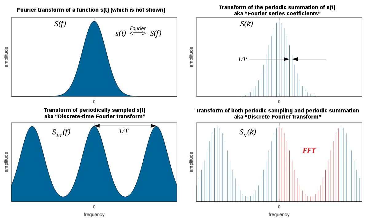
Discrete Fourier transform - Wikipedia
I coded a DFT Discrete Fourier Transform(DFT) program to see how fast it would run in Python. I don't read math well enough to code an FFT from a paper without having to work through it.
Search on Cooley Tukey FFT for the early math on the Fast Fourier Transform circa 1960s. It s one of mist important applied math techniques in technology and other areas.
FFTW s a common package and is open source.
n = 2^12 takes a few seconds, 2^14 about 60 seconds. The Python Numpy add on probably as an FFT function.
The DFT is essentially a digital correlation. The k loop in the code breaks down a sine wave into n parts and correlates it to the y the input signal. For a complex signal with many frequency components any frequency but the one being correlated in the k loop sums to zero.
Search on cross and auto correlation.
The number of points in he transform sets the frequency resolution at the cost of more time to run.
You can change frequencies on two sine waves and see how close they can be and be resolved.
The sampling frequency is set at 500 hertz, That makes the Nyquist frequency 250 hertz. Any frequency above 250 will alias. You can experiment with it and see how the alias occurs. 20 hz, 520 hz, 1020 hz will all show as 20 hz in the transformed spectrum.
The n point transform yields two mirror spectrums, so the first speed improvement s is running only n/2 points. The energy is spit between the two mirror spectrums, so the to get the true amplitude of a frequency the magnitude is multiplied by 2, and divided by n for the correlation average. Frequencies not being correlated average to zero.
mag[0] is frequency zero, the average value of the entire waveform.
It s a real transform, meaning the input signal has to be real not complex. A complex transform takes a little more work.
If you plot the y signal at 20 and 520 hz the plots will look the same, 20 hz. That is aliasing.
You can compare the experiential and the cos-sin form.
Change the delimiter on the save to a coma and it can be read into a spread sheet to plot. Or just look up the frequency pf interest in the file.
Code:
DFT
import math as m
import cmath

def save_nums(fname,delim,nrows,x,y):
        f = open(fname,'w')
        s = ""
        s += repr(n) + "\n"  # first line number of rows
        f. write(s)
        for i in range(nrows):
                s = ' ' # row string
                s += repr(x[i])
                s += delim
                s += repr(y[i])
                s += '\n'
                f.write(s)
        f.close()
        return 0


def dft(n,y,fs,f,mag):
    print("Start")
    n2 = int( n/2)
    print(n,"   ",n2)
    w = 2.*m.pi/n
    c2 = 2./n
    fsum = 0
    df = fs/n
    for freq in range(n2):
        f[freq] = fsum  # trasform frequency scaling
        fsum +=  df
        c3 = w * freq
        sum = 0. + 0.j  # complex number
        for k in range(n):
                sum += y[k]*cmath.exp(-1.j*c3*k)
                #sum += y[k]*( m.cos(c3*k) - 1j*m.sin(c3*k));
        if freq == 0:
                mag[freq] = sum.real/n # averge value of the waveform
        else:
                mag[freq] = c2 *abs(sum)
        if mag[freq] > 8 : print("%f   %f" %(f[freq],mag[freq]))
    print("Done")

def make_sin(n,y,t,f1,f2,a1,a2,os1,os2):
    tsum = 0
    dt = 1./float(fs)
    for i in range(n):
        t[i] = tsum
        y1 = a1*m.sin(2*m.pi*f1*tsum) + os1
        y2 = a2*m.sin(2*m.pi*f2*tsum) + os2
        y[i] = y1 + y2
        tsum += dt

n = pow(2,12)  # transform size power of 2
n2 = int(n/2)
y = n*[0]  # signal
f = n*[0]  # transform frequency bins, trasform plot x axis
mag = n *[0]  # #transforrm lines magnitude
t = n*[0]  # signal time, plot x axis
fs = 500  # sampling frequency
a1 = 10   # signal amplitude
a2 = 10
os1 = 0  # offset
os2 = 0
f1 = 40  # signal frequency
f2 = 200

make_sin(n,y,t,f1,f2,a1,a2,os1,os2)
dft(n,y,fs,f,mag)
save_nums("dfty.txt","            \t",n,t,y)
save_nums("dftm.txt","               \t ",n,f,mag)