The Calculus Thread

[steve_bank]

Pop quiz.

y(t) = A*sin(2*PI*f*t)

For f = 2 and A = 10, what is the equations of the lines tangent to the curve at t = PI/4 and t = PI?

 

[steve_bank]

Pop quiz.

y(t) = A*sin(2*PI*f*t)

For f = 2 and A = 10, what is the equations of the lines tangent to the curve at t = PI/4 and t = PI?

Correction

At t = 0 .25 and t = .01325

 

[lpetrich]

Here's a nice little calculus problem. Find

(d/dx) x^x

 

[steve_bank]

Here's a nice little calculus problem. Find

(d/dx) x^x

Nice. You got me I'd have to cogitate on it.

My first thought would be to try the chain rule but that mayl not work.

 

[Swammerdami]

Here's a nice little calculus problem. Find

(d/dx) x^x

x^x = e^{x⋅ln x}
The derivative of that is itself times derivative of x⋅ln x, which is ln x + 1.
So ... (d/dx) x^x = e^{x⋅ln x}⋅ (ln x + 1)

 

[lpetrich]

To visualize calculus operations:

• Differentiation = slope
• Integration = area

The fundamental theorem of calculus is that differentiation and integration are inverses of each other. But integration is much more difficult than differentiation.

Consider functions formed by arithmetic operations and power operations. A derivative is always that kind of function. But an integral is not necessarily that kind of function, even very simple integrals like

integral of 1/x over x

\( \displaystyle{ \int \frac{dx}{x} } \)

In fact, there are many functions that are defined as integrals and as solutions of differential equations, a generalization of integrals. Integral equations and integrodifferential ones also exist.

Numerous tables of integrals have been written over the last few centuries, and integration is a challenging problem for computer algebra:  Risch algorithm for instance. By comparison, computer-algebra differentiation is almost absurdly easy.

Wolfram Research has domain name integrals.com - it once had its own page, but it is now subsumed into Wolfram Alpha: Integral Calculator: Integrate with Wolfram|Alpha

 

[lpetrich]

Though infinite series are neither differentiation nor integration, they are nevertheless defined in much the same way, and many solutions of integrals and differential-equation are expressed as infinite series.

Is it common for calculus textbooks to have sections on infinite series?

Wikibooks is an open-content textbook site, and it has numerous textbooks in various states of completion. One of them is Calculus - Wikibooks, open books for an open world -- discussing differentiation, integration, differential equations, infinite series, etc.

Open content? Like open source in being freely available and freely modifiable.

 

[lpetrich]

One often wants to find numerical solutions, and there are a variety of ways of doing that.

For differentiation, one may naively do that by using the definition of it:

(f(x+h) - f(x))/h

That is inadequate, because when one expands f(x) in a Taylor series around h, one finds

f'(x) + (h/2)*f''(x) + (h²/6)*f'''(x) + ...

There is a way of increasing the accuracy of one's derivative. Since the second term is proportional to h, and since using -h would make it go in the opposite direction, one can take the average of these two results:

(f(x+h) - f(x-h))/(2h) = f(x) + (h²/6)*f'''(x) + O(h⁴)

One can go further with

(-f(x+2h) +4f(x+h) - 4f(x-h) + f(x-2h))/(6h) = f(x) + O(h⁴)

If one was to do numerical differentiation on some collected data, one will get a very noisy result. So to do that with collected data, one must first fit some curve to that data, and then differentiate that curve.

 

[steve_bank]

I remember basic series in first year calculus.

The derivative is defined as the limit at a point as +- dx goes to zero(can't do the actual notation). A limit of differences.

In the problem I posted the derivative of the function is the slope of the tangent line y = mx + b. You have m(slope), x, and y solve for b. Derivative of sine is cosine. I got the number wrong it should be .0625 resulting in PI/4 or 45 degrees . sin(PI/4) = cos(PI/4) = .707

The integral is the limit of sums as dx goes to zero. xdx being the area of a rectangle.

It may be more correct to say series solutions to integrals are an approximation. Many important integral forms do not have closed solutions. With high speed PCs numerical integration is easier.

The terms that link interline and derivative are derivative and antiderivative.

An antiderivative of a function f(x) is a function whose derivative is equal to f(x). That is, if F′(x)=f(x), then F(x) is an antiderivative of f(x)

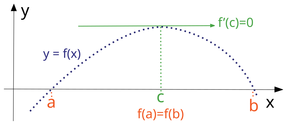
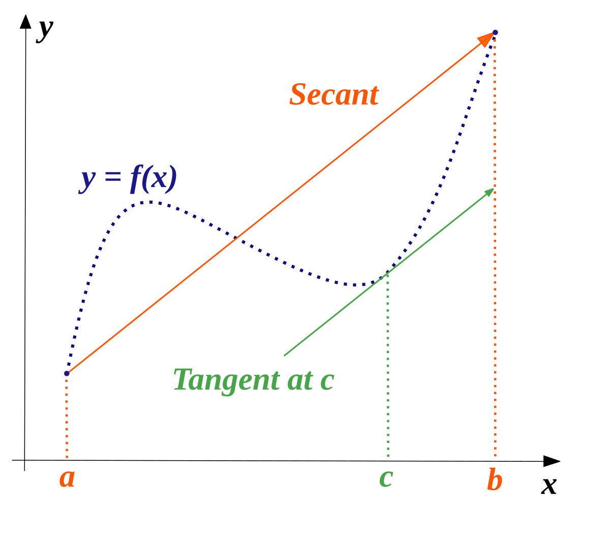
For something more inserting in basic calculus Mean Value Theorem and Rolle's Theorem. They are used tp prove other basic math in calculus. For the mathemcally inclibed.

Rolle's theorem - Wikipedia

en.wikipedia.org

Mean value theorem - Wikipedia

en.wikipedia.org

 

[steve_bank]

Here's a nice little calculus problem. Find

(d/dx) x^x

Nice. You got me I'd have to cogitate on it.

My first thought would be to try the chain rule but that mayl not work.

The soluions are easily found on the net....

 

[steve_bank]

Integro-differential equation - Wikipedia

en.wikipedia.org

Integro-differential equations are common in mechacal and elecrical engineering. It means you have to take both integrals and dervctives in the same equaion. Scrol down to apications in the link, RLC circuit.

Often non linear and are solved numercally with a 'solver' another topic.

 

[steve_bank]

Making the problem simpler.

What is the equation of the line tangent to y = sin(x) at x = %pi/4 (45 degrees) and pi (180 degrees)?

The equation of a line in point slope form is y = m*x +b where m is the slope and b is the offset.

The rate of change of a function at a point is the 1st derivative.
y = sin(x)
y' = cos(x)
x = pi/4
y = sin(pi/4) = .707
y' = cos(pi/4) = .707
y = m*x + b
.707 = .707*pi/4 + b
b = .707 - .707*pi/4 = .1517464
y = ,707* x + .152

Plotting the sin and the tangent line.

Plots tangent lines for sin(x) for xpt = 0 to pi.

//Scilab script
clear
clc
n = 1000
xpt = %pi/2  //x value
dt = %pi/n
x = [0:dt:%pi-dt]'
b = sin(xpt) - cos(xpt)*xpt
m = cos(xpt)
disp(b)
for i =  1:n
    ysin(i) = sin(x(i))
    yline(i) = m*x(i) + b
   end
w1 = scf(1)
clf(w1)
plot2d(x,ysin)
plot2d(x,yline)
xgrid

What is the tangent line at y = sin(pi)?

 

[lpetrich]

Numerical integration can also be done on a curve fitted to some data, and such integration is more generally useful, given the difficulty of finding many integrals.

Two simple algorithms, for integral of f(x) for x from a to b - \( \int_a^b f(x) \, dx \)

• Trapezoidal -- (b - a) * (f(a) + f(b))/2 -- \( (b-a) (f(a)+f(b))/2 \)
• Midpoint -- (b - a) * f((a+b)/2) -- \( (b-a) f((a+b)/2) \)

One can break a domain of integration into smaller segments and do either algorithm on each one. One can also use some fancier algorithm for each step, like Newton-Cotes integration (several equally-spaced points) or Gaussian integration (several variably-spaced points).

One can repeat this integration with more and more points, and reuse the previous calculations, checking on whether the result tends to converge.

One can have the help of interpolation, and the most general sort of polynomial interpolation is Lagrange interpolation:

y = sum over i of yi * product over j != i of (x - xi)/(xj - xi) -- \( \displaystyle{ y = \sum_i y_i \prod_{j \ne i} \frac{x - x_i}{x_j - x_i} } \)

But there is a way to calculate this interpolation efficiently. Create a pyramid of values starting with points 1, 2, ..., n. Create each new layer from sets of neighboring values in the previous ones: 1-2, 2-3, 3-4, ... (n-1)-n, 1-2-3, 2-3-4, ..., (n-2)-(n-1)-n, ...

 

[lpetrich]

Turning to differential equations, I will consider "ordinary" ones, ODE's, ones where there is a single independent variable. Those with more than one are "partial" ones, and they are more difficult.

Let us solve dy/dx = f(y) for x from 0 to h.

The simplest ODE-solution method is Euler's method:

ynew = y + h*f(y)

One can improve on it by using this result as an intermediate result, giving Heun's method:

yitmd = y + h*f(y)
ynew = y + (h/2)*(f(y) + f(yitmd))

There's a classic ODE solver, the Runge-Kutta fourth-order method, that is reasonably accurate for most of what one is likely to want to do. It is also easy to code.

k1 = h*f(y)
k2 = h*f(y + (1/2)*k1)
k3 = h*f(y + (1/2)*k2)
k4 = h*f(y + k3)
ynew = y + (1/6)*(k1 + 2*k2 + 2*k3 + k4)


There are similar methods with more points, and methods that will let one estimate the accuracy of one's solution from only the points that one has calculated.

If one's solution has evenly spaced points, one can use those points in linear multistep methods, using one method to come up with an estimate and another method to improve that estimate -- predictor-corrector methods.

There are various other sorts of ODE solvers, ones that are adapted to various sorts of problems, like Verlet and symplectic ones.

 

[steve_bank]

Take a look at the La Place Transform method of solving differential equations.

A common technique.

 

[steve_bank]

Take a look at the La Place Transform method of solving differential equations. A common technique.

 

[lpetrich]

The Laplace transform is a relative of the Fourier transform.

Fourier:
\( \displaystyle{ F(y) = \int_{-\infty}^{\infty} e^{i x y} f(x) \,dx ;\ f(x) =\frac{1}{2\pi} \int_{-\infty}^{\infty} e^{- i x y} F(y) \,dy } \)
Laplace:
\( \displaystyle{ F(s) = \int_0^\infty e^{-s t} f(t) \, dt ;\ f(t) = \frac{1}{2\pi i} \int_{c-i\infty}^{c+i\infty} e^{s t} F(s) \,ds } \)

 

[steve_bank]

A simple numerical integration of a 1st order linear differential equation via Euler's method. A simple series resonator capacitor circuit. Examples abound on the net.

The differential equation for a capacitor is i = C*dv/dt

i current through capacitor
C capacitance in farads
dv/dt change in capacitor voltage per change in time

A pure capacitance is linear, for a constant i the voltage change is a straight line.

Prearranging dv = i*dt/C

Euler's method assumes that over an interval dt the current is constant and dv a linear approximation

That leads into choice of dt the time step. Too short and there are unnecessary iterations, too long and you might miss short duration changes in the function. Accuracy vs execution time. An adaptibe algorithm might vary the time step proportional to the local rate of change of the function.

The equation for a series RC circuit is Vin(t) = i(t)*R + ∫i*dt/C
Vin applied voltage
Vc instantaneous capacitor voltage

The voltage across the capacitor is experiential.

//Scilab script
//Euler's Method  differntials
//series RC circuit charge
clear
clc
n = 20
integration_time = 1 //seconds
dt = integration_time/n  // time step
R = 1000  // reistor ohms
C = 100e-6  //capacitor microfarads
Vin = 1  // applied voltage
Time = 0  // time record
Vc = 0 //imital condition starting ca[acitor voltage
for j = 1:n
    v(j) = Vc  // capitor voltage at time t
    t(j) = Time
    Iresistor = (Vin - Vc)/R  //find  resistor current
    i(j) = Iresistor  // instantaneous current
    dv = dt*Iresistor/C  // find differntial change in voltade on cap
   Vc = Vc + dv  // update integral
    Time = Time + dt
end 
mprintf(" %f   %f   %.10f\n",t,v,i)   
w1 = scf(1)
clf(w1)
subplot(2,1,1)
plot2d(t,v)
xgrid
title"VOLTAGE"
subplot(2,1,2)
plot2d(t,i)
xgrid
title"CURRENT"

time, capacitor voltage, current

 0.000000   0.000000   0.0010000000
 0.050000   0.500000   0.0005000000
 0.100000   0.750000   0.0002500000
 0.150000   0.875000   0.0001250000
 0.200000   0.937500   0.0000625000
 0.250000   0.968750   0.0000312500
 0.300000   0.984375   0.0000156250
 0.350000   0.992188   0.0000078125
 0.400000   0.996094   0.0000039063
 0.450000   0.998047   0.0000019531
 0.500000   0.999023   0.0000009766
 0.550000   0.999512   0.0000004883
 0.600000   0.999756   0.0000002441
 0.650000   0.999878   0.0000001221
 0.700000   0.999939   0.0000000610
 0.750000   0.999969   0.0000000305
 0.800000   0.999985   0.0000000153
 0.850000   0.999992   0.0000000076
 0.900000   0.999996   0.0000000038
 0.950000   0.999998   0.0000000019

Given the speed of PCs I generally used this technique, small time step and a lot of iterations.

 

[steve_bank]

Comparing the actual integral to the numeral integration.

for j = 1:n
    v(j) = Vc  // capitor voltage at time t
    t(j) = Time
    va(j) = Vin*( 1 - %e^(-t(j)/(R*C)) )  // actual continuous time solution
    Iresistor = (Vin - Vc)/R  //find  resistor current
    i(j) = Iresistor  // instantaneous current
    dv = dt*Iresistor/C  // find differntial change in voltade on cap
   Vc = Vc + dv  // update integral
    Time = Time + dt
end 
mprintf(" %f   %f   %f   %.10f\n",t,v,va,i)

At n = 20 not a close approximation, at n = 50 better approximation.

t, numerical integration, actual integral

n = 20

 0.000000   0.000000   0.000000
 0.050000   0.500000   0.393469
 0.100000   0.750000   0.632121
 0.150000   0.875000   0.776870
 0.200000   0.937500   0.864665
 0.250000   0.968750   0.917915
 0.300000   0.984375   0.950213
 0.350000   0.992188   0.969803
 0.400000   0.996094   0.981684
 0.450000   0.998047   0.988891
 0.500000   0.999023   0.993262
 0.550000   0.999512   0.995913
 0.600000   0.999756   0.997521
 0.650000   0.999878   0.998497
 0.700000   0.999939   0.999088
 0.750000   0.999969   0.999447
 0.800000   0.999985   0.999665
 0.850000   0.999992   0.999797
 0.900000   0.999996   0.999877
 0.950000   0.999998   0.999925

n = 50

 0.000000   0.000000   0.000000
 0.020000   0.200000   0.181269
 0.040000   0.360000   0.329680
 0.060000   0.488000   0.451188
 0.080000   0.590400   0.550671
 0.100000   0.672320   0.632121
 0.120000   0.737856   0.698806
 0.140000   0.790285   0.753403
 0.160000   0.832228   0.798103
 0.180000   0.865782   0.834701
 0.200000   0.892626   0.864665
 0.220000   0.914101   0.889197
 0.240000   0.931281   0.909282
 0.260000   0.945024   0.925726
 0.280000   0.956020   0.939190
 0.300000   0.964816   0.950213
 0.320000   0.971853   0.959238
 0.340000   0.977482   0.966627
 0.360000   0.981986   0.972676
 0.380000   0.985588   0.977629
 0.400000   0.988471   0.981684
 0.420000   0.990777   0.985004
 0.440000   0.992621   0.987723
 0.460000   0.994097   0.989948
 0.480000   0.995278   0.991770
 0.500000   0.996222   0.993262
 0.520000   0.996978   0.994483
 0.540000   0.997582   0.995483
 0.560000   0.998066   0.996302
 0.580000   0.998453   0.996972
 0.600000   0.998762   0.997521
 0.620000   0.999010   0.997971
 0.640000   0.999208   0.998338
 0.660000   0.999366   0.998640
 0.680000   0.999493   0.998886
 0.700000   0.999594   0.999088
 0.720000   0.999675   0.999253
 0.740000   0.999740   0.999389
 0.760000   0.999792   0.999500
 0.780000   0.999834   0.999590
 0.800000   0.999867   0.999665
 0.820000   0.999894   0.999725
 0.840000   0.999915   0.999775
 0.860000   0.999932   0.999816
 0.880000   0.999946   0.999849
 0.900000   0.999956   0.999877
 0.920000   0.999965   0.999899
 0.940000   0.999972   0.999917
 0.960000   0.999978   0.999932
 0.980000   0.999982   0.999945

 

[steve_bank]

The flip side of integration, differentiation.

Derivative of sine is cosine.

//Scilab script
//derivative of a sine is cosine

clear
clc
_2PI = 2*%pi
f = 1
tmax = 2
n = 1000
dt = tmax/n
t = [0:dt:tmax]'
ys = sin(2*%pi*f*t)

for i = 1:n-1
    yd(i) = (ys(i+1)-ys(i))/dt  //dy/dt
end
 
w1 = scf(1)
clf(w1)
subplot(2,1,1)
plot2d(t,ys)
xgrid
title"SINE"
subplot(2,1,2)
plot2d(yd/_2PI)
xgrid
title"DERIVATIVE"