• Welcome to the new Internet Infidels Discussion Board, formerly Talk Freethought.

The Calculus Thread

When Isaac Newton and Gottfried Wilhelm Leibniz developed the calculus, they defined differential calculus with "infinitesimals", nonzero numbers that are closer to zero than any other nonzero number. That seemed nonsensical to some people, and in the early 19th century, mathematicians developed the concept of limits, making infinitesimals unnecessary.

Infinitesimals are well-defined in something called "nonstandard analysis", however. They can be defined as some number x times an infinitesimal unit e, where e2 = 0.

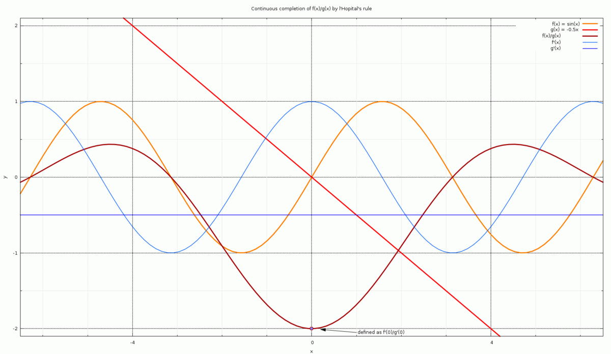
Here is the limit L of a function f(x) as x goes to a.

For some value eps, there is some value del such that for every x satisfying |x - a| < del, |f(x) - L| < eps.

This can be extended to infinite limits and limits of infinte series, and one can also do one-sided limits, limits from x > a or x < a.

For a positive infinite limit at some point:

For some value eps, there is some value del such that for every x satisfying |x - a| < del, f(x) > eps.

One can also do negative infinity, f(x) < eps, and both-directions and complex infinity, |f(x)| > eps.

For the limit for tending to positive infinity:

For some value eps, there is some value del such that for every x > del, |f(x) - L| < eps.

One can also do negative infinity, x < del, and both-directions and complex infinity, |x| > del.

One can combine these two types of infinite limits to find an infinite limit for tending to infinity.

Thus, one can define taking a derivative with a limit:

f'(x) = limit of (f(x+h) - f(x))/h as h tends to 0

instead of making h an infinitesimal.
 
For infinite sequences, a(1), a(2), ... one can define limits analogously. For limit L,

For some value eps, there is some value N such that for every n > N, |a(n) - L| < eps.

If there is such a limit, the sequence converges. For an infinite limit, the sequence diverges:

For some value eps, there is some value N such that for every n > N, |a(n)| > eps.

Convergence can be defined without an explicit limit, and a sequence with that property is a "Cauchy sequence":

For some value eps, there is some value N such that for every n, m > N, |a(n) - a(m)| < eps.

A nice feature of Cauchy convergence is that it enables defining real numbers as Cauchy sequences of rational numbers, since the limits do not have to be defined in whatever set the sequences members are defined in.

This is evident from sequences like 1, 1/2, 1/3, 1/4, ..., where all the members are positive yet with a limit of 0.

Cauchy sequences of real numbers are also real numbers, making real numbers Cauchy-closed.
 
To get numbers in general, one can do:
  • Natural numbers: Peano's axioms: 0 and its successors.
  • Integers: natural numbers with subtraction
  • Rational numbers: integers with division
  • Algebraic numbers: rational numbers with polynomial roots -- algebraically closed
  • Real numbers: rational numbers with Cauchy-series limits -- Cauchy-closed
  • Complex numbers: combinations of algebraic and real numbers -- algebraically and Cauchy closed
  • Computable numbers: sequences of rational numbers from running a Turing machine arbitrarily long
To be equivalent to a Turing machine, one must be able to do
  • Random access of arrays of arbitrary size
  • Arbitrary flow of control
In practice, one can't have infinite array size, but if one is only limited by how much memory one has, then a system will be Turing complete to within resource limits.

Alan Turing's universality theorem means that it's unnecessary to built special-purpose hardware for every computing problem, only Turing-complete general-purpose hardware, though one can build special-purpose hardware to improve performance.
 
The exponential function can be defined as this limit:

\( \displaystyle{ \exp x = \lim_{n \to \infty} \left( 1 + \frac{x}{n} \right)^n } \)

It's easy to show that this makes an infinite series:

\( \displaystyle{ \exp x = \sum_{n=0}^\infty \frac{x^n}{n!} } \)

From the infinte-series definition, it is easy to show that

exp(0) = 1
exp(x)*exp(y) = exp(x+y)

and from there, that exp(x) = ex where e = exp(1) ~ 2.7182818...

\( \displaystyle{ \exp x \exp y = \sum_{n=0,m=0}^{\infty,\infty} \frac{x^m y^n}{m! n!} = \sum_{n=0,k=0}^{\infty,n} \frac{x^k y^{n-k}}{k! (n-k)!} } \\ \displaystyle{ = \sum_{n=0}^\infty \frac{1}{n!} \sum_{k=0}^n \frac{n!}{k! (n-k)!} x^{k} y^{n-k} = \sum_{n=0}^\infty \frac{(x+y)^n}{n!} = \exp (x+y) } \)
 
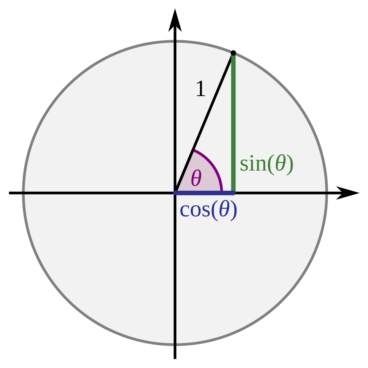
I'll now take on trigonometry. I'll start off with geometric definitions. For right triangle ABC, with the right angle at B and for angle a at BAC,

(AB) = (AC) * cos(a)
(BC) = (AC) * sin(a)
(AC) = (AB) * sec(a)
(BC) = (AB) * tan(a)

One can find some special values and trigonometric identities with these, like

\( sin 0 = 1 \\ \cos 0 = 1 \\ \sin^2 a + \cos^2 a = 1 \\ \sin (a+b) = \sin a \cos b + \cos a \sin b \\ \cos(a+b) = \cos a \cos b - \sin a \sin b \)

Let us now relate these trig functions to their angle. To do that, we use the area of a slice of a circle with radius r and angle a at the origin: S(r,a)

The variation with radius is easy. The area of a rectangle with side lengths a and b is a*b, and scaling both a and b gives r*a*r*b = r2 * (original area). Likewise the area of a triangle scales by that factor, and dividing a circle slice into small rectangles and/or triangles likewise gives scaling by r2

So S(r,a) = r2 * S(a)

For S(a), note that it has special value S(0) = 0 and that it is additive by angle: S(a+b) = S(a) + S(b). This makes

S = S0 * a

For convenience in what follows, I will set S0 = 1/2.
 
Next up is some inequalities found with areas.

Take a circle with origin O and shoot out two rays with angle a between them between 0 and 90d, and make three circles centered at 0. The first circle intersects the two rays at A and A', the second one at B and B', and the third one at C and C'. Choose the circle radii so that OAB' and OBC' are both right angles. Also choose the radius of the second circle to be 1. The first and third circles thus have radii cos(a) and sec(a).

This results in an area inequality

\( \displaystyle{ \frac12 a \cos^2 a < \frac12 \cos a \sin a < \frac12 a < \frac12 \sec a \tan a < \frac12 a \sec^2 a } \)

This gives us inequality

\( \displaystyle{ \cos a \sin a < \sin a < a < \tan a < \sec a \tan a } \)

Since tan(a) = sin(a)/cos(a), and cos(a) -> 1 as a -> 0, we find that sin(a) -> a as a -> 0.

Now use these results to find the derivatives of the sine and cosine functions. The other trigonometric functions' derivatives follow from these.

\( \displaystyle{ \frac{d}{da} \sin a = \cos a \lim_{h \to 0} \frac{\sin h}{h} + \sin a \lim_{h \to 0} \frac{\cos h - 1}{h} } \)

\( \displaystyle{ \frac{d}{da} \cos a = - \sin a \lim_{h \to 0} \frac{\sin h}{h} + \cos a \lim_{h \to 0} \frac{\cos h - 1}{h} } \)

The limits are
\( \displaystyle{ \lim_{h \to 0} \frac{\sin h}{h} = 1 ,\ \lim_{h \to 0} \frac{\cos h - 1}{h} = - \lim_{h \to 0} \frac{\sin^2 h}{h(1 + \cos h)} = 0 } \)

giving derivatives
(d/da) sin(a) = cos(a)
(d/da) cos(a) = - sin(a)
 
From these derivatives, one can find series expansions of these two trig functions:

\( \displaystyle{ \sin a = \sum_{n=0}^\infty \frac{ (-1)^n a^{2n+1}}{(2n+1)!} } \\ \displaystyle{ \cos a = \sum_{n=0}^\infty \frac{ (-1)^n a^{2n}}{(2n)!} } \)

Finally, one can show from the series expansions that

\( \displaystyle{ e^{i a} = \cos a + i \sin a } \)
 
Lagrange multipliers are a technique that very often proves useful. I don't know if they're introduced in basic calculus classes, but they're the first thing mentioned in a text on calculus of variations. It's been decades since I fired a Lagrange multiplier "in anger"; and my skills are horrendously rusty, but I tried to fashion a simple example without Googling "Interesting application of Lagrange multiplier." If too easy, you wouldn't need the technique.

Here's an example problem I came up with. I think solving without use of Lagrange multiplier may be quite tedious, but with the technique a few minutes should suffice.

Maximize f(x,y,z) = (xy + xyz) subject to the constraint that x + 2y + 3z = 15.
The obvious approach (though it won't work, due to the constraint) is to write
∂f(x,y,z)/∂x = 0​
∂f(x,y,z)/∂y = 0​
∂f(x,y,z)/∂z = 0​
That's three equations in three unknowns. But wait a minute! What about the fourth equation:
x + 2y + 3z = 15​
With FOUR equations we need a FOURTH unknown. Enter the Lagrange multiplier, usually denoted with λ.

It's simple to apply the technique. Instead of ∂/∂(x,y,z) (f(x,y,z)) = 0 write ∂/∂(x,y,z) (f(x,y,z) + λg(x,y,z)) = 0
where g(x,y,z) = 0 is the constraint; g(x,y,z) = x+2y+3z-15 in our example.

The technique can be applied with multiple constraints, e.g. for three constraints:
∂/∂(x,y,z) (f(x,y,z) + λ1g1(x,y,z) + λ2g2(x,y,z) + λ3g3(x,y,z)) = 0​

The proof that Lagrange multipliers work is called the Euler-Lagrange Theorem -- named after the two greatest mathematicians of the 18th century. (There may be several theorems with that same name.) The proof is a good exercise in working with (ε,δ).
 
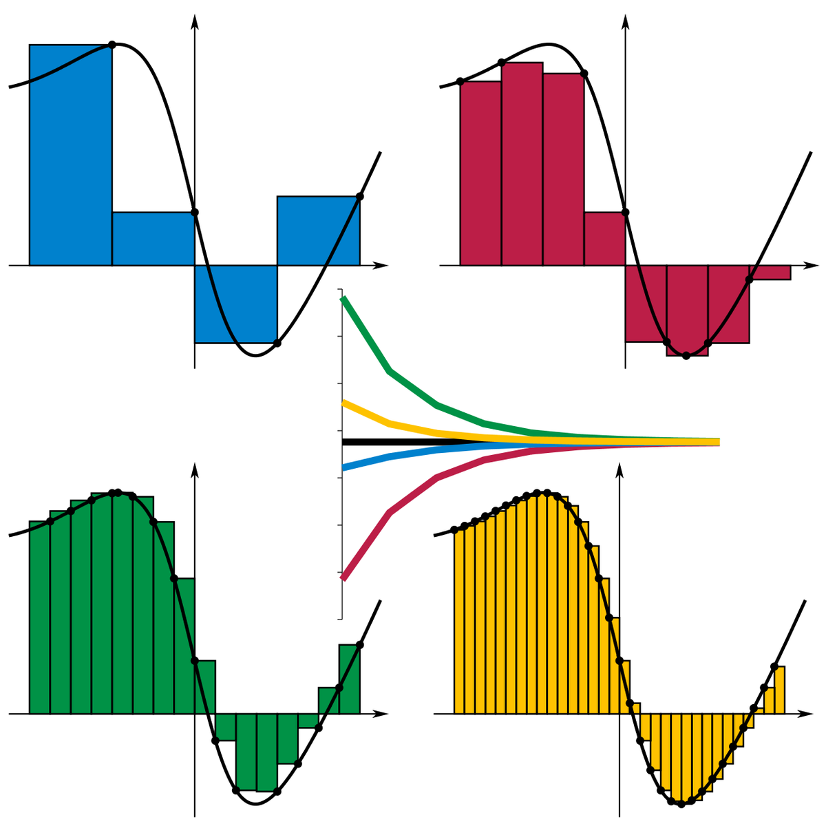
Riemann Sums or rectangular integration.

One of the main reasons I got my first computer was to go through texts and code problems to learn it.

Heuristic learning
a method of learning or solving problems that allows people to discover things themselves and learn from their own experiences

A common way to terminate iterative solutions is to exit when the relative change between two iterations is less than or equal to some value.


Interpreter tools like Scilab are good, but too slow for large sets of ietrations. I woud do ierations in C and use Scilab for post processing.

A useful fact to know is that the integral and derisive of e^x are e^x.
Riemann sums used to integrate e^x compared to the exact integral.

Code:
//reiman sums
clear
clc
 
lolim = 0  // integration limits
hilim = 5
nsums = 10  //initial resolution
max_iterations = 10
area_exact = %e^hilim - %e^lolim //acual integration
reltol = .001 //relatve chnange tolerance
for j = 1:max_iterations
    mprintf("%d\n",j)
    reimann_sum = 0  //zero integral
    dx = (hilim-lolim)/nsums
    x = [lolim:dx:hilim]
    for i = 1:length(x);y(i) = %e^x(i);end;
    for i = 1:nsums-1
        reimann_sum = reimann_sum + y(i) * dx
    end
    clear x y
    n(j) = nsums
    nsums = nsums * 10  //increase resolution by a fctor of 10
    rsum(j) = reimann_sum
    // end if relative change <= reltol
    if(j>1) then
            if((rsum(j)-rsum(j-1))/rsum(j) <= reltol)
                break
            end
   end
end
   
mprintf("Exact  %f\n",area_exact)
mprintf("%12.6f   %20d\n",rsum,n)


Code:
Exact  147.413159
Integral, Iterations
   68.609691                     10
  136.699792                    100
  146.306569                   1000
  147.302139                  10000
  147.402054                 100000
 
 List of Runge–Kutta methods - a big list

Euler (simplest):
0 ;
- ; 1

Midpoint:
0 ;
1/2 ; 1/2
- ; 0 , 1

Trapezoid (Heun):
0 ;
1 ; 1
- ; 1/2 , 1/2

Classic RK4:
0 ;
1/2 ; 1/2
1/2 ; 0 , 1/2
1 ; 0 , 0 , 1
- ; 1/6 , 1/3 , 1/3 , 1/6

Also has embedded methods, that make two results that can be compared, and implicit methods, which one solves iteratively, and which are useful for stiff problems.
 
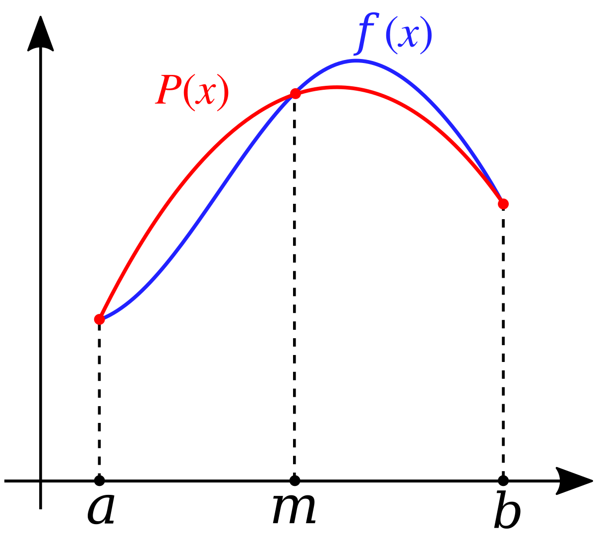
Newton divided-differences interpolation:  Newton polynomial

Divided differences of y(i) over x(i):

y(i) -- starting point
y(i,i+1) = (y(i+1) - y(i)) / (x(i+1) - x(i))
y(i,i+1,i+2) = (y(i+1,i+2) - y(i,i+1)) / (x(i+2) - x(i))
y(i,i+1,i+2,i+3) = (y(i+1,i+2,i+3) - y(i,i+1,i+2)) / (x(i+3) - x(i))
...

making a pyramid of values, starting at y(1) ... y(n) and ending at y(1,2,...,n)

The interpolation itself:

y(x) = y(1) + y(1,2)*(x-x1) + y(1,2,3)*(x-1)(x-2) + ...


Neville interpolation for point x:  Neville's algorithm
y(i) -- starting point
y(i,i+1) = ((x(i+1) - x)*y(i) + (x - x(i))*y(i+1)) / (x(i+1) - x(i))
y(i,i+1,i+2) = ((x(i+2) - x)*y(i,i+1) + (x - x(i))*y(i+1,i+2)) / (x(i+2) - x(i))
y(i,i+1,i+2,i+3) = ((x(i+3) - x)*y(i,i+1,i+2) + (x - x(i))*y(i+1,i+2,i+3)) / (x(i+3) - x(i))
...

making the same kind of pyramid of values, with y(1,2,...,n) being the interpolation result.


These two algorithms are mathematically equivalent to  Lagrange polynomial interpolation, but they require less computation, and they are numerically better behaved. For N points, they are all O(N2), and for Newton's method, once one has done some O(N2 precalculation, each point requires only O(N) of calculation.
 
 Linear multistep method - one can use previous points in a solution of an ordinary differential equation.

For solving dy/dx = f(x,y) I'll use f(i) = f(x(i),y(i)) for evenly spaced points x(i) with interval h.

The methods: y(i+1) = y(i) + h * (what's below)

Adams-Bashforth: explicit - multiplying f(i), f(i-1), f(i-2), ...
1
3/2 -1/2
23/12 -16/12 +5/12
55/24 -59/24 +37/24 -9/24
1901/720 -2774/720 +2616/720 -1274/720

Adams–Moulton: implicit - multiplying f(i+1), f(i), f(i-1), ...
1
1/2 +1/2
5/12 +8/12 -1/12
9/24 +19/24 -5/24 +1/24
251/720 +646/720 -264/720 +106/720

One can use them in predictor-corrector fashion, doing Adams-Bashforth, then Adams-Moulton.
 
I'll work the example problem with the Lagrange multiplier λ.

Lagrange multipliers are a technique that very often proves useful. ...

Maximize f(x,y,z) = (xy + xyz) subject to the constraint that x + 2y + 3z = 15.

It's simple to apply the technique. Instead of ∂/∂(x,y,z) (f(x,y,z)) = 0 write ∂/∂(x,y,z) (f(x,y,z) + λg(x,y,z)) = 0
where g(x,y,z) = 0 is the constraint; g(x,y,z) = x+2y+3z-15 in our example.
We start with four equations in four unknowns
∂(xy + xyz + λ(x+2y+3z-15) )) / ∂x = 0​
∂(xy + xyz + λ(x+2y+3z-15) )) / ∂y = 0​
∂(xy + xyz + λ(x+2y+3z-15) )) / ∂z = 0​
x+2y+3z-15 = 0​
Perform the indicated differentiations
y + yz + λ = 0​
x + xz + 2λ = 0​
xy + 3λ = 0​
Multiply by constants to make it easy to solve
6y + 6yz = -6λ (1)​
3x + 3xz = -6λ (2)​
2xy = -6λ (3)​
x + 2y + 3z = 15 (4)​
If there's a positive solution at all, then x≠0 and y≠0, because xy + xyz would otherwise not then be positive.
Combine (1) and (3); divide by 2y
3 + 3z = x (5)​
Combine (2) and (3); divide by x
3 + 3z = 2y (6)​
Plug (5) and (6) into (4)
3 + 3z + 3 + 3z + 3z = 15​
z = 1​
and then plug z=1 into (5) and (6).
x = 6​
y = 3​

This simple problem would be MUCH more tedious without the Lagrange multiplier. For more difficult problems the Lagrange multiplier is essential.
 
Oldies but goodies. With PCs and numerical solutions not much use any more.
Integration By Part, Trigonometric Substitution, and Simpson's Rule.

There was a time I had Simpson's Rule coded in a programmable hand held calculator. Useing had held calculators to solve diffeqs was common. Graphical calculators with simple strip printers were important in the day.

had a calculus teacher who had worked at a post war national lab as a staff mathematician, his specialty was integration. Somebody would walk into the math room with a problem. The group would work the problem in turn as an error check. Slide rules and mechanical calculators.

There used to be large wall hanging slide rules for improved precision.

Covered in basic calculus.


Simpson's rule is one of the  Newton–Cotes formulas along with the trapezoidal and midpoint rules.

Newton-Cotes formulas are for integral for x = a to b of f(x), and they can be either closed (the points containing endpoints) or open (the points offset from endpoints).

Closed:
sum for k = 0 to n of (b-a)*w(k)*f(a + h*k) where h = (b-a)/n

Half-Open:
sum for k = 0 to n of (b-a)*w(k)*f(a + h*(k+1/2)) where h = (b-a)/(n+1)

Open:
sum for k = 0 to n of (b-a)*w(k)*f(a + h*(k+1)) where h = (b-a)/(n+2)

for weights w, given as:

Closed:
(1/2) * {1, 1} -- trapezoidal rule
(1/6) * {1, 4, 1} -- Simpson's rule
(1/8) * {1, 3, 3, 1} -- Simpson's 3/8 rule
(1/90) * {7, 32, 12, 32, 7} -- Boole's rule

Half-Open:
1 * {1} -- midpoint rule
(1/2) * {1, 1}
(1/8) * {3, 2, 3}
(1/48) * {13, 11, 11, 13}

Open:
1 * {1} -- midpoint rule
(1/2) * {1, 1}
(1/3) * {2, -1, 2} -- Milne's rule
(1/24) * {11, 1, 1, 11}

Abramowitz and Stegun - Page index -- a big collection of math-related stuff: special functions, coefficients in various formulas, etc.
 
I decided to write a coefficients calculator for Newton-Cotes and multistep formulas in Python, though I could also do it in C++ with the help of some C++ fractions library. I've used one, and it's easy: it's a template library: Rational<integer>.

The multistep coefficients:

Explicit:
1 * {1}
(1/2) * {3, -1}
(1/12) * {23, -16, 5}
(1/24) * {55, -59, 37, -9}
(1/720) * {1901, -2774, 2616, -1274, 251}

Implicit:
1 * {1}
(1/2) * {1, 1}
(1/12) * {5, 8, 1}
(1/24) * {9, 19, -5, 1}
(1/720) * {251, 646, -264, 106, -19}

(missing term in previous post: -19/720)

For the Newton-Cotes formula, I've verified all the formulas in Abramowitz & Stegun and Wikipedia.
 
What I wrote:
Code:
#!python3
#
# Calculates numerical-integration coefficients:
# Newton-Cotes
# multistep ODE solving
#
# Args:
# What to calculate
# Index value (number of points, or that number + 1)
#
# What to calculate:
# NCCls - Newton-Cotes closed
# NCHfO - Newton-Cotes half-open
# NCOpn - Newton-Cotes open
# MSPrd - Adams-Bashforth (multistep predictor)
# MSCor - Adams-Moulton (multistep corrector)

from sys import argv, exit
from functools import reduce
from fractions import Fraction
from math import gcd, lcm

# Will do the calculations analytically,
# by manipulating polynomials as lists of coefficients
# coefficients for powers 0, 1, 2, ...
# Degree of polynomial is length - 1

# Multiply two polynomials
def PolyMult(poly1, poly2):
	# Polynomial degrees
	n1 = len(poly1)
	n2 = len(poly2)
	n = n1 + n2 - 1
	polyres = n*[0]
	for k1 in range(n1):
		for k2 in range(n2):
			polyres[k1+k2] += poly1[k1] * poly2[k2]
	
	return polyres

# Multiply a list of polynomials
def PolyMultList(polylist):
	return reduce(PolyMult, polylist, [1])

# Calculate Lagrange-interpolation coefficient polynomials
# and integrate them over (0, 1).
def LagrCoefIntegr(points):
	n = len(points)
	
	CoefItgrs = n*[0]
	
	for k in range(n):
		numlist = [ [-points[m],1] for m in range(n) if m != k]
		nlprod = PolyMultList(numlist)
		
		# Integral from 0 to 1
		nlpint = 0
		for m in range(n):
			nlpint += Fraction(1,m+1)*nlprod[m]
		
		denlist = [ points[k] - points[m] for m in range(n) if m != k]
		den = reduce(lambda x1, x2: x1*x2, denlist, 1)
		
		CoefItgrs[k] = nlpint/Fraction(den)
	
	return CoefItgrs

# Do the calculation for one set

if len(argv) <= 2:
	print("Not enough args")
	exit(0)

CoefType = argv[1]
CoefIndex = int(argv[2])

print("Coefficient type and index:", CoefType, CoefIndex)

n = CoefIndex
if CoefType == "NCCls":
	Coefs = [Fraction(k,n) for k in range(n+1)]
elif CoefType == "NCHfO":
	Coefs = [Fraction(1,n)*(k + Fraction(1,2)) for k in range(n)]
elif CoefType == "NCOpn":
	Coefs = [Fraction(k+1,n+1) for k in range(n)]
elif CoefType == "MSPrd":
	Coefs = [- k for k in range(n)]
elif CoefType == "MSCor":
	Coefs = [1- k for k in range(n)]
else:
	print("Unrecognized type:", CoefType)
	exit(0)

IntCoefs = LagrCoefIntegr(Coefs)

denoms = [coef.denominator for coef in IntCoefs]

alldenom = reduce(lcm,denoms)

numers = [coef.numerator * (alldenom // coef.denominator) for coef in IntCoefs]

allnumer = reduce(gcd,numers)

rednumers = [num // allnumer for num in numers]

print("Overall numerator & denominator, reduced coefficients")
print(allnumer, alldenom, rednumers)
 
 Gaussian quadrature

Instead of equally-spaced points, one selects points that are related to the roots of "orthogonal polynomials", with those points' weights being related to those polynomials' derivatives.

What kinds of orthogonal polynomials are there?

Take polynomials P(n,x) of degree n for independent variable x. Orthogonality:

integral for x from x1 to x2 of w(x)*P(n,x)*P(m,x) is nonzero only for n = m

for some weighting function w(x). The polynomials satisfy this differential equation in y as a function of x:

(x - x1)*(x2 - x)*y'' + (p1*x + p0)*y' + n*(n - 2*p1 - 1)*y = 0

and they and their derivatives satisfy some recurrence relations, Rodriguez formulas, generating functions, and series expansions.

The most general ones are  Jacobi polynomials

Interval: -1, 1
Weighting: w(x) = (1 - x)a * (1 + x)b
Differential equation: (1 - x2)*y'' + (b - a - (a+b+2)*x)*y' + n*(n + a + b + 1)*y = 0

For a = b, one finds the  Gegenbauer polynomials or ultraspherical ones. Taking c = a - 1/2,u

Interval: -1, 1
Weighting: w(x) = (1 - x2)c-1/2
Differential equation: (1 - x2)*y'' - (2c + 1)*y' + n*(n + 2c)*y = 0

For c = 1/2, one finds the  Legendre polynomials

The associated ones for additional parameter m have c = m + 1/2

For c = 0, one finds the  Chebyshev polynomials of the first kind:

T(n,x) = cos(n*arccos(x))

For c = 1, one finds the Chebyshev polynomials of the second kind:

U(n,x) = sin((n+1)*arccos(x))/sin(x)

For x1 = 0 and x2 = +oo, one finds the  Laguerre polynomials

Here are the generalized or associated Laguerre ones, or Sonine ones:

Interval: 0, +oo
Weighting: xc * e-x
Differential equation: x*y'' + (c + 1 - x)*y' + n*x = 0

The plain Laguerre polynomials have c = 0.

For x1 = -oo and x2 = +oo, one finds the  Hermite polynomials] With scaling factor k,

Interval: -oo, +oo
Weighting: e-k*x^2
Differential equation): y'' - 2k*x*y' + 2k*n*y = 0

There are two conventions for k:
  • Probabilist's: k = 1/2
  • Physicist's: k = 1

One can find the Laguerre and Hermite polynomials as limiting cases of the Jacobi ones for one or both of the limits sent to infinity, with each limit's associated exponent sent to infinity, and with the independent variable shifted and scaled as appropriate.
 
Back
Top Bottom